Xinmiao Lu* | Qiong Wu | Ying Zhou | Yao Ma | Chaochen Song | Chi Ma
© 2019 IIETA. This article is published by IIETA and is licensed under the CC BY 4.0 license (http://creativecommons.org/licenses/by/4.0/).
OPEN ACCESS
The k-means clustering (KMC) algorithm easily falls into the local optimum trap, if the initial cluster centers are not reasonable. To solve the problem, this paper puts forward a dynamic swarm firefly algorithm based on chaos theory and max-min distance algorithm (FCMM). Firstly, the number of cluster centers, k, and their positions were determined by the maxi-min distance algorithm (MM). Then, a chaotic space was constructed by tent map based on the cluster centers, and the cluster centers were updated through chaotic search. In this way, the initial cluster centers are no longer concentrated in a small area, and the algorithm is not prone to the local optimum trap. The simulation results show that the FCMM successfully avoids the local optimum trap, achieves efficient classification of the initial dataset, and converges to the global optimal solution in an accurate manner.
k-means clustering (KMC), max-min distance algorithm (MM), firefly algorithm (FA), chaos theory
With the dawn of the big data era, great progress has been made in the field of data mining. As a classical method of data mining and analysis [1, 2], cluster analysis enjoys a huge application potential in pattern recognition, indoor positioning and statistics. The improvement of clustering accuracy has long been a research hotspot, aiming to satisfy the growing demand for data accuracy [3, 4].
Since the traditional k-means clustering (KMC) algorithm is easily affected by the initial cluster centers and abnormal data [5, 6], many scholars have attempted to optimize the initial cluster centers of the traditional KMC in the light of feature correlation [7, 8] and develop clustering algorithms based on adaptive weight [9, 10]. The firefly algorithm (FA), a stochastic optimization algorithm mimicking the firefly behaviors, has been widely adopted to optimize the KMC for its ability to improve the accuracy of clustering algorithms. The FA is highly robust, easy to operate and supports parallel processing [11, 12], providing an effective solution to various optimization problems.
Considering the fact that the KMC, relying heavily on the initial cluster centers, is prone to fall into the local optimum trap, Pan et al. [13] proposed a firefly partitional clustering algorithm based on adaptive step length, which avoids the local optimum trap by replacing the fixed step length of the KMC with adaptive step length. Wang et al. designed a novel niche firefly partitional clustering algorithm to enhance population diversity [14]. Chen et al. [15] introduced a weighted Euclidean distance to optimize the initial cluster centers of the KMC, utilizing the strong global search ability and easy implementation feature of the FA.
The above FA-optimized KMC algorithms can achieve better clustering effect when the cluster centers are given. However, none of them clearly defines how to determine the number of cluster centers, k. The firefly partitional clustering algorithm based on adaptive step length has a small step length in the late stage of optimization, which easily causes slow convergence. What is worse, the dataset cannot jump out of the current cluster center, thus reducing the clustering accuracy.
To solve the above problems, this paper puts forward a dynamic swarm FA based on chaos theory and max-min distance algorithm (FCMM). Firstly, the max-min distance algorithm (MM) was adopted to determine the number of cluster centers, k, and the positions of the initial cluster centers. Then, the chaotic tent map, featuring uniform ergodicity and fast iteration, was employed to set up a chaotic search space with the initial cluster centers as the reference points. Next, the initial cluster centers were optimized by chaotic tent search, such that the algorithm can jump out of the local optimum trap and converge to the global optimum rapidly. Finally, the position update formula of the FA was used to allocate the sample points other than the cluster centers to suitable clusters, putting an end to the clustering process.
2.1 The KMC
The essence of the KMC is to classify a given dataset $X=\left\{X_{1}, X_{2}, \ldots, X_{n}\right\}$ into k classes $\left\{C_{1}, C_{2}, \ldots, C_{k}\right\}$. The classic KMC contains the following steps: First, selecting k objects randomly from the dataset X and taking them the initial cluster centers $C_{j}(j=1,2, \ldots, k)$ of k classes; Then, computing the Euclidean distance is computed between each remaining object $X_{i}(i=1,2, \dots, n)$ and each cluster center, and allocating each remaining object to the nearest class $C_{j}$; Next, recalculating the mean value of all objects in each class, and taking it as the new cluster center [16]. The above steps are repeated until the cluster center of each class no longer changes.
Definition 1. Euclidean distance
The Euclidean distance is the linear distance between two points in Euclidean space [17]. In an m-dimensional space, the Euclidean distance between the samples $X_i$ and $X_j$ can be expressed as:
$d\left(X_{i}, X_{j}\right)=\sqrt{\sum_{k=1}^{m}\left(X_{i k}-X_{j k}\right)^{2}}$ (1)
The KMC determines the similarity between samples based on the Euclidean distance.
2.2 The FA
Inspired by firefly motions, the FA computes the objective function value and relative attractiveness of each firefly according to its position and light intensity. The lighter fireflies move towards the brighter ones, using the position update formula. The moving distance depends on the attractiveness. The optimization of the FA adheres to the following three principles:
(1) Any two fireflies can attract each other, regardless of their gender.
(2) The attractiveness of a firefly is negatively correlated with its distance to another firefly and positively correlated with its light intensity. The lighter fireflies are attracted by and move towards the brighter ones, while the brightest firefly moves randomly.
(3) The light intensity of a firefly depends on the objective function value at its position.
Definition 2. The light intensity I of each firefly can be defined as:
$I \propto-f\left(x_{i}\right), 1 \leq i \leq n$ (2)
$I=I_{0} \exp \left(-\gamma * r_{i j}\right)$ (3)
where, $f\left(x_{i}\right)$ is the objective function; $\mathcal{X}_{i}$ is the spatial position of firefly i ; $I_{0}$ is the maximum light intensity; γ is a constant representing the light intensity absorption; $r_{i j}$ is the Euclidean distance between $X_{i}$ and $X_{j}$.
Definition 3. The attractiveness of each firefly can be defined as:
$\beta=\beta_{0} \exp \left(-\gamma * r_{i j}^{2}\right)$ (4)
where, $\beta_{0}$ is the maximum attractiveness?
Definition 4. The position update formula can be described as:
$x_{i}(t+1)=x_{i}(t)+\beta\left(x_{j}(t)-x_{i}(t)\right)+\alpha \varepsilon_{i}$ (5)
where, α is the initial step length; $\varepsilon_{i}$ is a random factor obeying the Gaussian distribution.
After initializing the cluster centers, the traditional KMC can be optimized with the randomness and global search ability of the FA. The FA-based optimization simulates the KMC process as the mutual attraction between fireflies, classifies the remaining objects accurately and speeds up the global convergence of the KMC. However, there are two defects with this optimization approach:
(1) No algorithm is available to determine the value of k, the number of cluster centers. If improperly selected, the k value may severely affect the clustering accuracy and computing complexity.
(2) The optimal clustering results correspond to the extreme points of the objective function, i.e. the cluster centers are close to local minimum points. Therefore, the algorithm easily falls into the local optimum trap.
To overcome these defects, this paper puts forward a dynamic swarm FA based on chaos theory and uses it to improve the KMC. The proposed FA draws on the sensitivity and ergodicity of chaotic mapping to initial values [18].
3.1 Determination of k by the MM
Like the traditional KMC, the MM allocates the sample points to cluster centers based on the nearest neighbor principle according to the Euclidean distance. The difference between the two algorithms lies in the determination of k. Instead of directly giving the k value, the MM selects a random object $X_{i}$ from the sample points as the first cluster center, computes the Euclidean distances of the remaining objects to $X_{i}$ by formula (1), and takes the object the furthest away from $X_{i}$ as the new cluster center. These steps are repeated until no new cluster center emerges, yielding the k value.
The MM is implemented in the following steps:
Step 1. Input θ (0<θ<1) and select the initial cluster center $Z_{1}=x_{1}$.
Step 2. Generate a new cluster center.
(1) Compute the Euclidean distance $D_{i 1}$ between each point and $Z_1$, and take the $x_k$ corresponding to $D_{k 1}=\max \left\{D_{i 1}\right\}$ as the new cluster center $Z_{2}$;
(2) Compute the Euclidean distances Di1 and Di2 between each point and cluster centers $Z_{1}$ and $Z_{2}$. If $D_{k 1}=\max \left\{D_{i 1}\right\} D D_{l}=\max \left\{\min \left(D_{i 1}, D_{i 2}\right)\right\}, i=1,2, \ldots n$ and $D_{l}>\theta * D_{12}$, take $x_l$ as the third cluster center $Z_3$.
Note that $D_{12}$ is the distance between $Z_1$ and $Z_2$:
$D_{i 1}=\left\|x_{i}-Z_{1}\right\|=\sqrt{\sum_{i=1}^{d}\left|x_{i}-Z_{1}\right|^{2}, D_{i 2}}=\left\|x_{i}-Z_{2}\right\|$
(3) If $Z_{3}$ exists, judge if $D_{j}=\max \left\{\min \left(D_{i 1}, D_{i 2}, D_{i 3}\right)\right\}$, i=1,2,...n. If yes and $D_{l}>\theta * D_{12}$ determine the fourth cluster center. Repeat the above process until $D_{l} \leq \theta * D_{12}$.
Step 3. Count the total number of cluster centers k.
The clustering results of the MM rely heavily on the selection of parameters and the first cluster center. If the sample distribution is not known in advance, repeated tests are needed for this algorithm to achieve a good clustering effect. As a result, this paper only uses the MM to determine the value of k.
3.2 Optimization of cluster centers with chaos theory
The random, ergodic and regular chaotic variables were introduced to improve the FA-optimized KMC, whose cluster centers often fall near local minimum points, aiming to enhance the global search ability and avoid the local minimum trap.
The logistic chaotic map faces obvious uneven ergodicity when the r value falls between 0 and 1, which suppresses the algorithm efficiency. Shan Liang et al. proved that the tent map outperforms logistic map in convergence speed and ergodic evenness, because the chaotic sequence generated by the tent map is more helpful to algorithm optimization [19].
(1) Tent chaotic sequence
The tent map can be expressed as:
$x_{t+1}=\left\{\begin{array}{c}{2 x_{t}, 0 \leq x_{t} \leq \frac{1}{2}} \\ {2\left(1-x_{t}\right), \frac{1}{2} \leq x_{t} \leq 1}\end{array}\right.$ (6)
Through dyadic transform, the tent map can be rewritten as:
$x_{t+1}=\left(2 x_{t}\right) \bmod 1$ (7)
The tent chaotic sequence is generated through the following steps:
Step 1. Randomly generate an initial value $x_0$ not in the range of (0.20,0.40,0.60,0.80) and denote it as $z, z(1)=x_{0}, i=j=$1.
Step 2. Iteratively generate a sequence x by formula (7).
Step 3. Implement Step 2 if x(i)=[0,0.25,0.5,0.75] or x(i)=x(i-k), (k=[0,1,2,3,4]).
Step 4. Change the initial value for iteration by x(i)=z(j+1), replace j with j+1, and implement Step 2.
Step 5. If the maximum number of iterations has been reached, terminate the iteration and save the sequence x.
(2) Chaotic search
The proposed FCMM generates a tent chaotic sequence based on the best-known local optimal solution, and jumps out of the local optimum trap through tent search, thereby converging to the global optimal solution.
Specifically, the distances $D_{i x}$ between all cluster centers $C_{i}(i=1,2, \dots k)$ and the current cluster center $C_x$ were ranked in descending order. Then, the smallest n classes (30% of all cluster centers) $C_{i 1}, C_{i 2}, \ldots, C_{i n}$ and $C_x$ were selected, and the maximum $X^{j} \max$ and minimum $X^{j} \min$ of the n+1 classes in the j-th dimension were computed, forming a new chaotic search space. After that, a chaotic sequence was generated based on cluster center $X_x$ of $C_x$, and used for chaotic search. The optimal solution obtained through the search was taken as the new cluster center.
Assuming that $C_x$ is the cluster center, $X_{k}=\left\{x_{k 1}, x_{k 2}, \dots x_{k d}\right\}$ and $x_{k j} \in\left[X_{\min }, X_{\max }\right]$, then the main steps of tent chaotic search can be explained as:
Step 1. Map $X_{x}$ to (0,1) by $z_{k j}^{0}=\left(x_{k j}-X_{\min }^{j}\right) /\left(X_{\max }^{j}-X_{\min }^{j}\right)$, where $k=1,2, \ldots, n, j=1,2, \ldots, D$.
Step 2. Substitute the above formula into formula (7) for tent map, and iteratively generate the chaotic variable sequence $Z_{k j}^{m}\left(m=1,2, \dots, C_{\max }\right)$b, where, $C_{\max }$ is the maximum number of iterations for the chaotic search [11].
Step 3. Restore $z_{k j}^{m}$ to the neighborhood of the original solution space by formula (8), producing a new $V_k$:
$v_{k j}=x_{k j}+\left(X_{\max }^{j}-X_{\min }^{j}\right) *\left(2 z_{k j}^{m}-1\right) / 2$ (8)
Step 4. Compute the light intensity $F\left(v_{k}\right)$ of $v_{k}$, compare it with the local optimal light intensity $F\left(x_{k}\right)$, and save the better solution.
Step 5. If the number of iterations has reached $C_{\max }$, terminate the search; otherwise, return to Step 2.
3.3 Basic steps of the FCMM
Step 1. Initialize the parameters: the total number of objects N, the light intensity absorption coefficient γ, the step length α, the maximum number of iterations for chaotic search $C_{\max }$, the maximum light intensity I and the maximum attractiveness $β_0$.
Step 2. Determine the number of cluster centers k by the MM, and record the position of the initial cluster center obtained by the MM.
Step 3. Construct the chaotic search space based on the cluster centers by tent map.
Step 4. Update the position of the initial cluster center by tent map until no new cluster center emerges.
Step 5. Consider cluster centers as fireflies with the highest light intensity, compute the Euclidean distances between remaining objects and each cluster center, and assign different light intensities to these objects by formula (3).
Step 6. If $I_{i}>I_{j}$, then firefly j has a smaller objective function value than firefly i, i.e. j is in a superior position than i. In this case, i is attracted by and moves towards j. Determine the movement pattern by formula (4) and update the firefly positions by formula (5).
Step 7. Repeat Step 6 until all fireflies have been allocated to their respective cluster centers.
Step 8. Output the results.
Three experiments were carried out to verify the effectiveness of the FCMM. The first experiment compares the clustering effects of the FCMM with the KMC and the FA; the second experiment tests the clustering accuracy and convergence speed of the three algorithms on the UCI datasets; the third experiment contrasts the clustering results of the FCMM with the firefly partitional clustering algorithm based on adaptive step length (Algorithm 1) and the KMC improved by weighted Euclidean distance (Algorithm 2).
4.2 Results analysis
(1) The first experiment
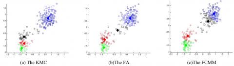
There are 200 samples scattering across the solution space. The number of cluster centers k was determined as 4 by the MM. Since the FA parameter setting has a great impact on experimental results, this paper obtains the parameter combination that leads to the most frequent occurrences of the optimal solution through parallel tests. A series of combinations between the step length α and the light intensity absorption coefficient γ were enumerated, and compared based on 30 sets of test results. Finally, the optimal parameters were determined as the maximum attractiveness $β_0$=100, the light intensity absorption coefficient γ=1, the step length α=0.06, the maximum number of iterations $C_{\max }$ =50, the maximum light intensity I=100, and θ=0.4. Using these parameters, the clustering results of the three algorithms are obtained as Figure 1.
As shown in Figure 1, the KMC clearly fell into the local optimum trap, as some of its cluster centers concentrated in a small area. The FA’s cluster centers were more distributed evenly than those of the KMC, but still need to be improved. The FCMM achieved better clustering effect than the KMC and the FA, evidenced by the uniform distribution of the cluster centers and the avoidance of the local minimum trap.
(2) The second experiment
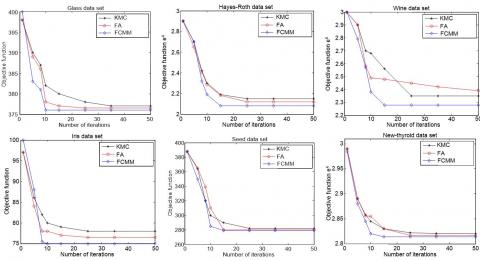
The KMC, FA and FCMM were tested independently on six datasets, using the same parameters as the first experiment. The mean clustering accuracy of each algorithm is given in Table 1, and the convergence curve of each algorithm is presented in Figure 2.
Table 1. The mean clustering accuracy of each algorithm (%)
|
Dataset |
KMC |
FA |
FCMM |
|
Iris |
87.93 |
91.13 |
92.16 |
|
Wine |
56.85 |
70.23 |
72.15 |
|
Seed |
86.97 |
88.07 |
90.46 |
|
Glass |
54.05 |
57.18 |
63.12 |
|
Hayes-Roth |
77.32 |
81.06 |
82.35 |
|
New-thyroid |
72.34 |
79.63 |
80.28 |
Figure 1. Clustering effects of the three algorithms
Figure 2. Convergence curves of the three algorithms on six datasets
Table 1 shows that the FCMM improved the mean clustering accuracy by 7.51 % and 2.2 % from the levels of the KMC and the FA, respectively, owing to the determination of the k value by the MM and the optimization of cluster centers by the chaotic theory. It can be seen from Figure 2 that the FCMM converged to the global optimal solution faster than the KMC and the FA, without sacrificing the clustering accuracy.
(3) The third experiment
This experiment mainly compares the clustering accuracy and runtime of the FCMM with those of Algorithm 1 and Algorithm 2.
Table 2 demonstrates that the FCMM achieved much higher clustering accuracy than the two contrastive algorithms, despite the relatively long runtime. The time complexity of the FCMM is attributable to the analysis on the initial cluster center by the MM.
Table 2. Comparison of results via the different algorithms
|
Data set |
Algorithm 1 |
Algorithm 2 |
FCMM |
|||
|
Clustering accuracy (%) |
Runtime (s) |
Clustering accuracy (%) |
Runtime (s) |
Clustering accuracy (%) |
Runtime (s) |
|
|
Iris |
91.49 |
8.342 |
91.22 |
9.234 |
92.16 |
8.34 |
|
Wine |
70.43 |
14.432 |
70.71 |
13.832 |
72.15 |
13.725 |
|
Seed |
89.70 |
9.232 |
89.52 |
8.342 |
90.46 |
8.282 |
|
Glass |
60.70 |
18.345 |
62.45 |
17.532 |
63.12 |
17.425 |
|
Hayes-Roth |
81.46 |
11.243 |
81.28 |
10.734 |
82.35 |
10.432 |
|
New-thyroid |
79.98 |
11.344 |
79.01 |
10.232 |
80.28 |
10.109 |
The KMC may easily fall into the local optimum trap, if the initial cluster centers are not suitable. To solve the problem, this paper designs a novel algorithm, the FCMM, that optimizes the KMC in two aspects: the number of initial cluster centers, k, and the position of cluster centers. Our way to determine the k value can effectively reduce the impact of k on the clustering algorithm. In addition, the positions of cluster centers were updated through chaotic search, based on the FA-optimized KMC. The chaotic map weakens the impacts of initial clustering position on the clustering effect, and fully utilizes the global search ability and fast convergence of the FA, making it possible to avoid the local optimum trap and converge to global optimal solution rapidly. The clustering effect of the FCMM was compared with that of other clustering algorithms and tested on several UCI datasets. The results show that the FCMM can achieve fast convergence, accuracy clustering and avoid the local optimum trap, when it is applied to cluster a few amounts of data.
[1] Esfahani, R.K., Shahbazi, F., Akbarzadeh, M. (2019). Three-phase classification of an uninterrupted traffic flow: A k-means clustering study. Transportmetrica B-Transport Dynamics, 7(1): 546-558. https://doi.org/10.1080/21680566.2018.1447409
[2] Huynh, P., Yoo, M. (2016). VLC-based positioning system for an indoor environment using an image sensor and an accelerometer sensor. Sensors, 16(6): 783. https://doi.org/10.3390/s16060783
[3] Franti, P., Sieranoja, S. (2019). How much can k-means be improved by using better initialization and repeats. Pattern Recognition, 93: 95-112. https://doi.org/10.1016/j.patcog.2019.04.014
[4] Wu, J., Yu, Z.J., Zhuge, J.C., Xue, B. (2016). Indoor positioning by using scanning infrared laser and ultrasonic technology. Optics & Precision Engineering, 24(10): 2417-2423. https://doi.org/10.3788/OPE.20162410.2417
[5] Fadaei, A., Khasteh, S.H. (2019). Enhanced k-means re-clustering over dynamic networks. Expert Systems with Applications, 132: 126-140. https://doi.org/10.1016/j.eswa.2019.04.061
[6] Yayan, U., Yucel, H., Yazici, A.G. (2016). A low cost ultrasonic based positioning system for the indoor navigation of mobile robots. Journal of Intelligent & Robotic Systems, 78(3-4): 541-552. https://doi.org/10.1007/s10846-014-0060-7
[7] Bai, L., Liang, J.Y., Guo, Y.K. (2018). An ensemble clusterer of multiple fuzzy k-means clusterings to recognize arbitrarily shaped clusters. IEEE Transactions on Fuzzy Systems, 26(6): 3524-3533. https://doi.org/10.1109/TFUZZ.2018.2835774
[8] Wang, T. (2012). Novel sensor location scheme using time-of-arrival estimates. IET Signal Processing, 6(1): 8-13. https://doi.org/10.1049/iet-spr.2010.0305
[9] Lithio, A., Maitra, R. (2018). An efficient k-means-type algorithm for clustering datasets with incomplete records. Statistical Analysis and Data Mining, 11(6): 296-311. https://doi.org/10.1002/sam.11392
[10] Jiang J.,Zheng X., Chen Y. (2013). A distributed RSS-based localization using a dynamic circle expanding mechanism. IEEE Sensors Journal, 13(10): 3754-3766. https://doi.org/10.1109/JSEN.2013.2258905
[11] Franti, P., Sieranoja, S. (2018). K-means properties on six clustering benchmark datasets. Applied Intelligence, 48(12): 4743-4759. https://doi.org/10.1007/s10489-018-1238-7
[12] Fang, S.H., Lin, T.N. (2010). A dynamic system approach for radio location fingerprinting in wireless local area networks. IEEE Transactions on Communications, 58(4): 1020-1025. https://doi.org/10.1109/tcomm.2010.04.090080
[13] Pan, X.Y., Chen, X.J., Li, A. (2017). Firefly partition clustering algorithm based on self-adaptive step. Application Research of Computers, 34(12): 3576-3579.
[14] Wang, C., Lei, X.J. (2014). New partition clustering algorithm of niching firefly. Computer Engineering, 40(5): 173-177. https://doi.org/10.3969/j.issn.1000-3428.2014.05.036
[15] Chen, X.X., Wei, Y.Q., Ren, M. (2018). Weighted K-means clustering algorithm based on firefly algorithm. Application Research of Computers, 35(2): 466-470.
[16] Garcia, J., Crawford, B., Soto, R. (2018). A k-means binarization framework applied to multidimensional knapsack problem. Applied Intelligence, 48(2): 357-380. https://doi.org/10.1007/s10489-017-0972-6
[17] Santhi, V., Jose, R. (2018). Performance analysis of parallel k-means with optimization algorithms for clustering on spark. Distributed Computing and Internet Technology, 10722: 158-162. https://doi.org/10.1007/978-3-319-72344-0_12
[18] Daniel, R., Rao, K.N. (2018). EEC-FM: Energy efficient clustering based on firefly and midpoint algorithms in wireless sensor network. KSII Transactions on Internet and Information Systems, 12(8): 3683-3703.
[19] Shan, L., Qiang, H., Li, J. (2005). Chaotic optimization algorithm based on tent map. Control and Decision, 20(2): 179-182.