Yanling Zhu* | Chunguang Xu | Dingguo Xiao
© 2019 IIETA. This article is published by IIETA and is licensed under the CC BY 4.0 license (http://creativecommons.org/licenses/by/4.0/).
OPEN ACCESS
To remove the noise in the echo signals of ultrasonic pulse-echo testing, this paper puts forward a denoising algorithm based on the generalized S transform (GST) and singular value decomposition (SVD). Firstly, the ultrasonic echo signals were subjected to the GST, yielding the time-frequency matrix of the signals. Next, the matrix was taken as the Hankel matrix, and went through the SVD. The threshold for singular values to be zeroed was determined by the ratio between singular entropy increments. After zeroing the singular values representing the noise, the resulting denoised 2D time-frequency matrix was subjected to the inverse GST, generating the denoised echo signals. Our method was applied to denoise the simulated ultrasonic echo signals with different signal-to-noise ratios (SNRs), and compared with the wavelet soft thresholding (WST) method. The comparison show that our method outperformed the WST, especially in denoising the signals with low SNR. In addition, a scanning acoustic microscopy (SAM) system was designed for the experimental verification of our method. The C-scan image with our method was much better than that without our method. Hence, our method was proved feasible and effective.
echo signals, generalized S transform (GST), singular value decomposition (SVD), c-scan image
During ultrasonic pulse-echo testing, the echo signals from the material attenuate significantly with the increase in testing frequency. The attenuation can be mitigated by increasing the gain setting. However, a high transmission gain may also amplify the noise. In addition, the noise intensity of the ultrasonic echo signals tends to change with the transmission distance of the ultrasonic wave and the property of the medium. Thus, the received echo signals will have a low signal-to-noise ratio (SNR), and the noise will form multiple peaks in the time domain. These phenomena severely hamper the positioning and extraction of the peak and amplitude of the echo signals from the interfaces of the measured material.
Currently, the ultrasonic signals are mainly denoised by short-time Fourier transform (STFT), wavelet transform (WT), various improved WTs, adaptive filtering (AF), and empirical mode decomposition (EMD). Each method has its unique strengths and defects in ultrasonic signal denoising. For example, the STFT is not suitable to process non-stationary signals, in that, once the window function is determined, the shape of the window can no longer be adjusted, while the window position on the phase plane can still be modified [1]. The WT has a certain ability to denoise ultrasonic signals, but needs to go through a complex process to obtain the wavelet threshold and threshold function. Moreover, the WT may distort the original signals, leading to discrete and oscillating signals [2-4]. The AF relies on the selection of the reference signal, which is not always correlated with the noise signals [5-6]. The EMD can decompose the original signals adaptively. But the decomposition is limited to the time domain, and the decomposed natural mode function faces signal-noise aliasing [7-9].
The singular value decomposition (SVD) denoising is a nonlinear filtering method that can effectively eliminate noises [10-11]. This is because the singular value, an intrinsic feature of the matrix, can remain stable, rotation invariant and proportional invariant in pattern recognition. The SVD is adopted to denoise ultrasonic echo signals in this research. The key to SVD denoising of ultrasonic echo signals lies in the construction of a suitable Hankel matrix. This matrix can be derived from the time-domain components of the original signals or the WT or EMD results of the original signals [12-14]. Nonetheless, the Hankel matrix thus obtained is unable to effectively characterize the time-frequency characteristics of the useful signals, or distinguish between the singular values of useful signals and noise, failing to achieve the denoising objective.
The generalized S transform (GST) offers a way to solve the problem. The GST combines the characteristics of the STFT and the WT: a high frequency-domain resolution in the low frequency band, and a high time-domain resolution in the high frequency band. The GST can adjust the time- and frequency- domain resolutions of the echo signals, such that the energy of the useful signals and that of the noise distribute in different time-frequency domains. Moreover, the GST also supports loss-free inverse transform [15-18]. If it is applied to the echo signals, the GST will output a 2D time-frequency matrix, laying the basis for a Hankel matrix that effectively reflects the time-frequency characteristics of the original signals.
In this paper, the GST and the SVD, which integrates information entropy, into a denoising method for ultrasonic echo signals. Firstly, the GST was performed on the echo signals from the interfaces of the target, outputting a time-frequency matrix. Next, the matrix was taken as the Hankel matrix for the SVD, and subjected to singular entropy decomposition. The decomposed matrix went through the inverse GST, producing the denoised echo signals. The proposed denoising method was adopted to process the simulated signals and the actual echo signals from the interfaces of a silicon wafer, and compared with the traditional denoising method: wavelet soft thresholding (WST). The results show that our method is both effective and superior. Finally, the feasibility of our method was verified through the application to the echo signals in an ultrasonic C-scan image.
For the 1D continuous signal x(t), the S transform can be defined as [19]:
$S(\tau, f)=\frac{|f|}{\sqrt{2 \pi}} \int_{-\infty}^{\infty} x(t) e^{-\frac{f^{2}(\tau-t)^{2}}{2}} e^{-j 2 \pi f t} d t$ (1)
The Fourier transform of the said signal can be expressed as:
$X(f)=\int_{-\infty}^{\infty} x(t) e^{-j 2 \pi f t} d t$ (2)
The time-domain integral of the S transform (1) can be described as:
$\int_{-\infty}^{\infty} S(\tau, f) d \tau=\int_{-\infty}^{\infty}\left\{\int_{-\infty}^{\infty} x(t) \frac{|f|}{\sqrt{2 \pi}} e^{-\frac{f^{2}(t-\tau)^{2}}{2}} e^{-j 2 \pi f t} d t\right\} d \tau=\int_{-\infty}^{\infty} x(t) e^{-j 2 \pi f t} d t=X(f)$ (3)
where, X(f) is the FT of signal x(t). Thus, the S transform is essentially a type of the FT. The inverse S transform can be derived from the FT:
$\int_{-\infty}^{\infty} X(f) e^{j 2 \pi f t} d f=\int_{-\infty}^{\infty}\left(\int_{-\infty}^{\infty} S(\tau, f) d t\right) e^{j 2 \pi f t} d f=x(t)$ (4)
Suppose the Gaussian window function w(t, f):
$w(t, f)=\frac{|f|}{\sqrt{2 \pi}} e^{-\frac{f^{2} t^{2}}{2}}$ (5)
satisfies
$\int_{-\infty}^{\infty} w(t, f) d t=1$ (6)
Introducing parameters a and b into (5) to adjust the time- and frequency-domain resolutions, then w(t, f) can be transformed as:
$w(t, f, a, b)=\frac{a|f|^{b}}{\sqrt{2 \pi}} e^{-\frac{a^{2} f^{2} t^{2}}{2}}$ (7)
Substituting (7) to (1), the GST of the signal can be obtained as:
$S(\tau, f, a, b)=\frac{a|f|^{b}}{\sqrt{2 \pi}} \int_{-\infty}^{\infty} x(t) e^{-\frac{a^{2} f^{2 b}(t-\tau)^{2}}{2}} e^{-j 2 \pi f t} d t$ (8)
2.2 The SVD of the 2D time-frequency matrix
The SVD denoising can effectively eliminate the Gaussian white noise in the original signal. In this paper, the 2D time-frequency matrix of the ultrasonic echo signals is obtained through the GST, and then denoised by the SVD.
Let f (tj) and σ(tj) be the discrete time sequences of the ultrasonic echo signals and the noise, respectively. Then, the actually received signals can be illustrated as:
$x\left(t_{j}\right)=f\left(t_{j}\right)+\sigma\left(t_{j}\right), \cdot(j=0,1,2, \cdots N-1)$ (9)
Performing the GST on (9), we have:
$\begin{align} & S[p,q]=\sum\limits_{j=0}^{N-1}{x({{t}_{j}})}\frac{a{{\left| q \right|}^{b}}}{\sqrt{2\pi }N}{{e}^{-\frac{{{a}^{2}}{{q}^{2b}}{{(p-j)}^{2}}}{2{{N}^{2}}}}}{{e}^{-\frac{i2\pi ja{{q}^{b}}}{N}}} \\ & =\sum\limits_{j=0}^{N-1}{f({{t}_{j}})}\frac{a{{\left| q \right|}^{b}}}{\sqrt{2\pi }N}{{e}^{-\frac{{{a}^{2}}{{q}^{2b}}{{(p-j)}^{2}}}{2{{N}^{2}}}}}{{e}^{-\frac{i2\pi ja{{q}^{b}}}{N}}}+\sum\limits_{j=0}^{N-1}{\sigma ({{t}_{j}})}\frac{a{{\left| q \right|}^{b}}}{\sqrt{2\pi }N}{{e}^{-\frac{{{a}^{2}}{{q}^{2b}}{{(p-j)}^{2}}}{2{{N}^{2}}}}}{{e}^{-\frac{i2\pi ja{{q}^{b}}}{N}}} \\ \end{align}$ (10)
${{A}_{(pq)j}}=\sum\limits_{j=0}^{N-1}{\frac{a{{\left| q \right|}^{b}}}{\sqrt{2\pi }N}}{{e}^{-\frac{{{a}^{2}}{{\left( p-j \right)}^{2}}{{q}^{2b}}}{2{{N}^{2}}}}}{{e}^{-\frac{ij2\pi a{{q}^{b}}}{N}}}$, $p,q=0,1,2,\cdots N-1$ (11)
where A(pq)j can be written as the matrix below:
$A_{(p q) j}=\left[\begin{array}{cccc}{A_{11}} & {A_{12}} & {\cdots} & {A_{1 N}} \\ {A_{21}} & {A_{22}} & {\cdots} & {A_{2 N}} \\ {\vdots} & {\vdots} & {\cdots} & {\vdots} \\ {A_{N 1}} & {A_{N 2}} & {\cdots} & {A_{N N}} \\ {A_{(N+1) 1}} & {A_{(N+1) 2}} & {\cdots} & {A_{(N+1) N}} \\ {\vdots} & {\vdots} & {\cdots} & {\vdots} \\ {A_{(p q) 1}} & {A_{(p q) 2}} & {\cdots} & {A_{(p q) N}}\end{array}\right]$ (12)
The A(pq)j is the time-frequency matrix obtained through the GST of the original signals. Each column is a time point of signal sampling, and each row is a frequency of the signals. Then, A(pq)j was taken as the Hankel matrix of the SVD, and subjected to the SVD. According to the singular value theorem, the matrix SÎRN×N must satisfy:
${{S}_{N\times N}}={{U}_{N\times l}}{{\Lambda }_{l\times l}}V_{l\times N}^{T}$ (13)
where UN×l is the time-domain characteristics of the echo signals; Vl×N is the frequency-domain characteristics of the echo signals; Λl×l is the diagonal matrix:
$\Lambda=\left|\begin{array}{cccc}{\beta_{1}} & {0} & {\cdots} & {0} \\ {0} & {\beta_{2}} & {0} & {\vdots} \\ {\vdots} & {0} & {\ddots} & {0} \\ {0} & {\cdots} & {0} & {\beta_{l}}\end{array}\right|$ (14)
where β1, β2…βl are the singular values of matrix S (β1≥β2≥…≥βl≥0). The singular values reflect the size of the main components of the echo signals. Large singular values represent useful signals, while small ones represent noise signals. The echo signals can be denoised by setting the small signals to zero and reconstructing the signals. The number of small singular values to be zeroed directly affects the effect of SVD denoising of the echo signals. If too many singular values are zeroed, some useful characteristics will not be contained in the reconstructed signals; if too few singular values are zeroed, the denoising will not be effective. In this paper, the threshold for singular values to be zeroed is determined by the ratio between singular entropy increments.
The singular values, obtained through the GST of the echo signals, were treated as the probability distribution sequence of the time-frequency information of the signals. The size of information entropy, a measure of sequence complexity, can be viewed as the uniformity of the probability distribution sequence [20]. Then, the m-th order singular entropy Em can be defined as:
${{E}_{m}}=\sum\limits_{j=1}^{m}{\Delta {{E}_{j}}}$, $m\le l$ (15)
$\Delta {{E}_{m}}=\sum\limits_{j=1}^{m}{-\left( {{{\beta }_{j}}}/{\sum\limits_{j=1}^{l}{{{\beta }_{j}}}}\; \right)}\log \left( {{{\beta }_{j}}}/{\sum\limits_{j=1}^{l}{{{\beta }_{j}}}}\; \right)$ $m\le l$ (16)
where ΔEj is the increment of the j-th order singular entropy.
The increments of the singular values of adjacent two orders (ΔEm and ΔEm+1) were computed. Then, the ratio between the two singular value increments ΔEm+1/ΔEm, denoted as γ, was taken as the threshold to determine which of β1, β2…βl in matrix Λ need to be zeroed.
To verify our method, ultrasonic echo signals were simulated by:
$x(t)=A_{i} e^{-\alpha\left(t-\tau_{i}\right)^{2}} \times \cos \left(2 \pi f_{i}\left(t-\tau_{i}\right)\right)+n(t)$ (i=1,2,3…) (17)
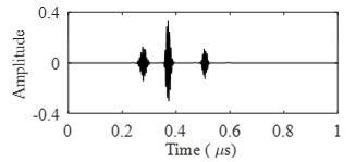
where Ai is the amplitude of an echo signal; α is the broadband factor; fi is the center frequency of an echo signal; τi is the time of arrival (TOA) of the echo signal from an interface of the target (i=1,2). The parameters of the echo signals for simulation were configured as: A1=10, α=300(MHz)2, f1=f2=100MHz, τ1=0.4μs, A2=8 and τ2=0.6μs.
The noiseless ultrasonic echo signals (Figure 1(a)) were added Gaussian white noises with the SNRs of 25, 15 and 5db, respectively. The resulting noisy signals are shown in Figures 1(b), 1(c) and 1(c), respectively. For comparison, our method and the WST method were applied to denoise the three types of noisy signals.
Figure 1. Noiseless echo signals and noisy echo signals with different SNRs
The denoising effects of the two methods on the simulated echo signals were evaluated by the SNR:
$S N R=10 \lg \frac{\sum_{i=1}^{N} S^{2}(t)}{\sum_{i=1}^{N}(X(t)-S(t))^{2}}$ (18)
where X(t) and S(t) are the original noisy signals and the denoised signals; N is the length of a signal.
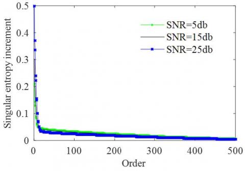
The increments of the singular values of adjacent two orders (ΔEm and ΔEm+1) were computed by (16). Then, the ratio between the two singular value increments γ was taken as the threshold to determine which of β1, β2…βl in matrix Λ need to be zeroed. In this way, the relationship between the singular entropy increment (ΔE) and the order of singular entropy was determined for ultrasonic echo signals with different SNRs (25, 15 and 5db).
As shown in Figure 2, the lower the SNR, the smaller the ΔE at a small order, and the greater the ΔE at a large order. With the increase in the order, the ΔE of all noisy signals, whichever the SNR, gradually decreased and became stable. The γ was also stabilized with the stabilization of ΔE.
Figure 2. Relationship between the singular entropy increment and the order of singular entropy
Figure 3. Denoising results at the SNR of 25db
The threshold for singular value zeroing was set to γ=0.8, which can retain all useful signals and remove all noise signals of the simulated echo signals. If ΔEm+1/ΔEm>0.8, the singular values β1…βm were kept, while βm+1…βl were set to zero, creating a new diagonal matrix. Substituting the matrix into (13), the denoised 2D time-frequency matrix could be obtained. Next, the denoised ultrasonic echo signals were obtained through inverse GST on the denoised 2D time-frequency matrix.
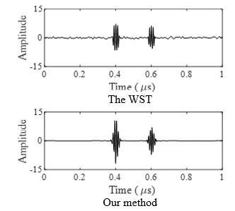
The denoising results of the three types of noisy signals are presented in Figures 3~5, respectively. For the noisy signals with low SNRs, the WST results still contained lots of noise. The denoising effect of this method is obviously undesirable. By contrast, our method managed to remove the noises and output smooth denoised signals, under the same condition.
Figure 4. Denoising results at the SNR of 15db
Figure 5. Denoising results at the SNR of 5db
Table 1 compares the SNRs of the signals denoised by the WST and our method. The comparison show that the WST could effectively remove the noises when the simulated echo signals have relatively high SNRs, but the denoising effect decreased with the SNR. The SNRs of the signals denoised by our method were much higher than those of the signals denoised by the WST, especially when the simulated echo signals have relatively low SNRs. The simulation results show that our method is an effective way to eliminate the noise from echo signals with low SNR.
Table 1. Comparison of the SNRs of the signals denoised by the WST and our method
|
method |
evaluation indicator |
25db |
15db |
5db |
|
WST |
SNR/dB |
27.26 |
16.76 |
7.64 |
|
Our method |
SNR/dB |
28.46 |
19.48 |
12.90 |
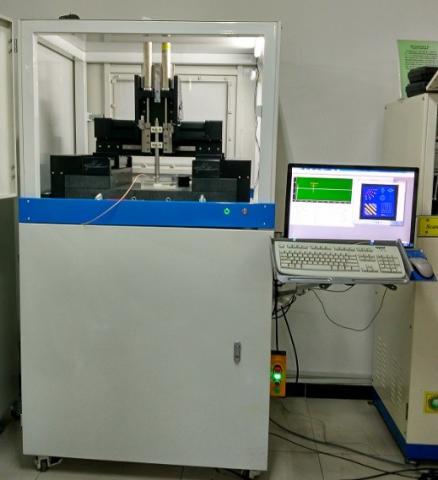
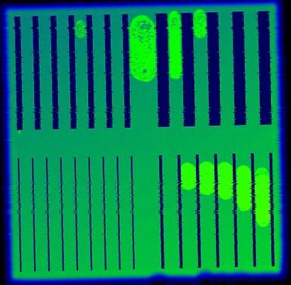
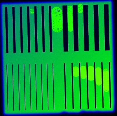
As shown in Figure 6, a scanning acoustic microscopy (SAM) system was designed for the experimental verification of our method. C-scan is the main working mode of the SAM system. Here is how the C-scan works: For a material, any change to the interior uniformity may alter its acoustic impedance. The incident acoustic wave will be partially reflected by the material. The remaining wave will penetrate the sample or interface (e.g. gain boundary, crack, cavity and delamination). These changes are reflected on the amplitude and phase of the echo signals received by the transducer. The structure of a profile in the sample can be displayed in real time, if the waveform data (e.g. peak and time) of each vertical incident point on the sample are shown in different colors or gray values.
Figure 6. The SAM system
Figure 7. The silicon wafer and the internal structure of the sample
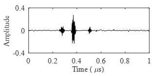
Figure 8. The ultrasonic echo signals from the interfaces inside the sample
The central frequency of the ultrasonic transducer was 100MHz, silicon wafer was selected as the targets, and the sampling frequency was set to 5GHz. The silicon wafer (10mm×10mm×0.5mm) is square on the upper and lower surfaces. Before the experiment, several 150μm-deep grooves with different widths were carved on the silicon wafer by laser etching. Then, the etched silicon wafer was covered with another silicon water of the same size, and the two wafers were bonded into a closed structure. The silicon wafer and the internal structure of the sample are shown in Figure 7.
Figure 8 shows the echo signals from the interfaces inside the sample measured in the experiment. Due to the high testing frequency, the noise in the echo signals was magnified under the high transmission gain. The received signals had a low SNR and multiple peaks, making it hard to the peak and amplitude of the echo signals.
Figure 9. The results of the WST
Figure 10. The results of our method
Figure 11. The C-scan image without our method
Figure 12. The C-scan image with our method
The denoising results of the WST (Figure 9) indicate severe distortion of the denoised signals. The denoising results of our method are presented in Figure 10. In this figure, the peaks of denoised signals were clear, and the time and amplitude of the signals could be extracted accurately. The comparison verifies the effectiveness of our method.
The SAM system was adopted to perform C-scans of the internal structure of the sample, with or without our method. Without our method, the echo signals from the internal interfaces of the sample were noisy, leading to blurred edges of the internal structure in the C-scan image (Figure 11). With our method, the noise in the echo signals was eliminated, and the internal structure and edges were clear in the C-scan image (Figure 12). The C-scan image obtained by our method facilitates the analysis on the interfaces and internal structure of silicon.
To remove the noise in the echo signals of ultrasonic pulse-echo testing, this paper puts forward a denoising algorithm based on the GST and SVD, which can eliminate the noise in both time- and frequency- domains. The 2D time-frequency matrix, obtained through the GST of ultrasonic echo signals, was subjected to the SVD. Among the SVD results, the large singular values represent useful signals, while small ones represent noise. Then, the threshold for singular values to be zeroed is determined by the ratio between singular entropy increments. During the experiment, the ultrasonic echo signals only contained the first two singular values, which greatly simplifies the denoising process. Our method was applied to denoise simulated ultrasonic echo signals, and the echo signals from the interfaces within a silicon sample. Both simulation and experimental results show that the signals denoised by our method had high SNRs, and that our method achieved better denoising effect than the WST when the original signals have a low SNR. Finally, the SAM system was adopted to perform C-scans of the internal structure of the sample, with or without our method. The results indicate that the C-scan image with our method was much better than that without our method.
The future research will tackle the following issues: (1) The effects of time- and frequency-domain factors a and b in the window function of the GST on the denoising results; (2) The denoising performance of our method on echo signals from complex interfaces (e.g. nonuniform coating) and the echo signals after multiple superpositions.
[1] Apostoloudia, A., Douka, E., Hadjileontiadis, L.J., Rekanos, I.T., Trochidis, A. (2007). Time–frequency analysis of transient dispersive waves: A comparative study. Applied Acoustics, 68(3): 296-309. https://doi.org/10.1016/j.apacoust.2006.02.002
[2] Jian, X., Guo, N., Dixon, S. (2005). Ultrasonic weak bond evaluation in ic packaging. Measurement Science and Technology, 17(10): 2637-2642. https://doi.org/10.1088/0957-0233/17/10/015
[3] Siqueira, M.H.S., Gatts, C.E.N., Da Silva, R.R. (2004). The use of ultrasonic guided waves and wavelets analysis in pipe inspection. Ultrsonics, 41(10): 785-797. https://doi.org/10.1016/j.ultras.2004.02.013
[4] Lee, U., Kim, S. (2006). Identification of multiple directional damages in a thin cylindrical shell. International Journal of Solids and Structures, 43(9): 2723-2743. https://doi.org/10.1016/j.ijsolstr.2005.03.077
[5] Keji, Y. (2005). An adaptive filter based on artificial neural net and its application in ultrasonic testing. Chinese Journal of Scientific Instrument, 26(8): 813-817. https://doi.org/10.3321/j.issn:0254-3087.2005.08.011
[6] Song, W., Wang, X., Li, M. (2007). Study on the denoising method for the electromagnetic ultrasonic echoes from multiple interfaces. Acta Acustica, 32(3): 226-231. https://doi.org/10.3321/j.issn:0371-0025.2007.03.005
[7] Kopsinis, Y., Mclaughlin, S. (2009). Development of EMD-based denoising methods inspired by wavelet thresholding. IEEE Transactions on Signal Processing, 57(4): 1351-1362. https://doi.org/10.1109/tsp.2009.2013885
[8] Haddad, S., Bouhadjera, A., Grimes, M., Benkedidah, T. (2011). A New ultrasonic signal processing scheme for detecting echoes of different spectral characteristics in concrete using empirical mode decomposition. Russian Journal of Nondestructive Testing, 47(9): 642-649. https://doi.org/10.1134/S106183091109004X
[9] Sharma, G.K., Kumar, A., Jayakumar, T. (2015). Ensemble empirical mode decomposition-based methodology for ultrasonic testing of coarse grain austenitic stainless steels. Ultrasonics, 57: 167-178. https://doi.org/10.1016/j.ultras.2014.11.008
[10] Gan, J., Zhang, Y. (2003). A study of singular value decomposition of face image matrix. Neural Networks and Signal Proeessing, 1: 197-199. https://doi.org/10.1109/ICNNSP.2003.1279245
[11] Cai, H., Xu, C., Zhou, S. (2015). Study on the thick-walled pipe ultrasonic signal enhancement of modified S-transform and singular value decomposition. Mathematical Problems in Engineering, 52(3): 351-363. https://doi.org/10.1155/2015/312620
[12] Li, Y., Wang, H., Chen, J. (2007). Research of noise reduction of underwater acoustic signals based on singular spectrum analysis. Systems Engineering and Electronics, 29(4): 524-527. https://doi.org/10.3321/j.issn:1001-506X.2007.04.006
[13] Liu, J.G., Li, Z.S., Liu, D. (2006). Features of underwater echo extraction based on SWT and SVD. Acta Acustica, 31(2): 167-172. https://doi.org/10.3321/j.issn:0371-0025.2006.02.012
[14] Zeng, X., Zhou, X., Yang, C. (2016). Ultrasonic defect echoes identification based on empirical mode decomposition and S-transform. Transactions of the Chinese Society for Agricultural Machinery, 47(11): 414-420. https://doi.org/10.6041/j.issn.1000-1298.2016.11.056
[15] Mansinha, L., Stockwell, R.G., Lowe, R.P. (1997). Pattern analysis with two-dimensional spectral localisation: Applications of two-dimensional S transforms. Physica A, 239(1-3): 286-295. https://doi.org/10.1016/s0378-4371(96)00487-6
[16] McFadden, P.D., Cook, J.G., Forster, L.M. (1999). Decomposition of gear vibration signals by the generalised S transform. Mechanical Systems and Signal Processing, 13(5): 691-707. https://doi.org/10.1006/mssp.1999.1233
[17] Pinnegar, C.R., Mansinha, L. (2003). The S-transform with windows of arbitrary and varying shape. Geophysics, 68(1): 381-385. https://doi.org/10.1190/1.1543223
[18] Schimmel, M., Gallart, J. (2005). The inverse S-transform in filters with time-frequency localization. Ieee Transactions on Signal Processing, 53(11): 4417-4422. https://doi.org/10.1109/tsp.2005.857065
[19] Stockwell, R.G., Mansinha, L., Lowe, R.P. (1996). Localization of the complex spectrum: The S transform. Ieee Transactions on Signal Processing, 44(4): 998-1001. https://doi.org/10.1109/78.492555
[20] Shannon, C.E. (1948). A mathematical theory of communication. Bell Labs Technical Journal, 1948(27): 379-433. https://doi.org/10.1002/j.1538-7305.1948.tb00917.x