Jin Ren* | Songyang Huang| Wei Song| Jun Han
© 2019 IIETA. This article is published by IIETA and is licensed under the CC BY 4.0 license (http://creativecommons.org/licenses/by/4.0/).
OPEN ACCESS
Considering the high accuracy needed for indoor positioning, this paper develops a novel indoor positioning algorithm for the wireless sensor network (WSN) in the following steps. First, the RSSIs of the network nodes were sampled and analyzed, and the excess errors were filtered to enhance positioning accuracy. Next, the initial position was iteratively obtained by the weighted centroid algorithm, and a correction matrix was developed to improve the Taylor series expansion (TSE), and the final position was determined through improved TSE iteration. The proposed positioning method was verified through simulation.
wireless sensor network (WSN), received signal strength indicator (RSSI), indoor positioning, Taylor series expansion (TSE), positioning accuracy
With the rapid development of mobile communication and terminals, the global positioning system (GPS), despite its excellent outdoor positioning effect, cannot fully support small-scale indoor location-aware services, owing to the complex channel environment and fast signal attenuation [1-3].
One of the solutions to the above problem is to develop a wireless local area network (LAN) with low cost and small power based on the wireless sensor network (WSN) technology. The WSN is an emerging technique integrating sensing, communication and distributed processing. Through the cooperation between its nodes, the network can capture and process the real-time information of multiple objects in the monitoring area, and transmit the processed information to interested users.
Node positioning technologies like the WSN takes positioning algorithm as the premise. The main positioning algorithms are based on field orientation, time different of arrival (TDoA), angle of Arrival (AoA), or received signal strength indicator (RSSI), or the coupling of these bases [4-6]. Thanks to its low hardware cost and simple implementation, the RSSI-based positioning algorithm becomes a research hotspot. In actual application, the proper position algorithm should be selected according to the specific environment and requirement.
In this paper, a novel indoor positioning algorithm is developed for the WSN in the following steps. First, the RSSIs of the network nodes were sampled and analyzed, and the excess errors were filtered to enhance positioning accuracy. Next, the initial position was iteratively obtained by the weighted centroid algorithm, and the correction matrix was improved by Taylor series expansion (TSE), and the final position was determined through iteration. The proposed positioning method was verified through simulation.
In the indoor environment, electromagnetic wave signals are affected by the propagation path, which is different from the propagation in free space. The distance between two nodes in the WSN can be estimated by the signal strength of the sending node and the signal strength at the receiving node, i.e. the RSSI. The RSSIs in wireless transmission can be explained by the shadowing model [7, 8]:
${{\left[ p\left( d \right) \right]}_{dBm}}={{\left[ p\left( {{d}_{0}} \right) \right]}_{dBm}}-10n\lg \left( \frac{d}{{{d}_{0}}} \right)+{{X}_{dBm}}$ (1)
where, p(d) is the RSSI of the receiving node separated from the sending node by a distance of d; p(d0) is the RSSI of the receiving node separated from the sending node by the reference distance d0; n is the path loss index; X is the cover factor. The path loss index depends on the external environment, and should be determined through actual measurement. The cover factor obeys the Gaussian random distribution and averages at zero.
In practice, the shadowing model is often simplified. For convenience, the reference distance can be set to 1m. Then, the $[p(d)]_{dBm}=A-10n lg(d)$ can be calculated by:
$RSSI=A-10n\lg \left( d \right)$ (2)
The above equation can be rewritten as:
$d\text{=1}{{\text{0}}^{\frac{A-RSSI}{10n}}}$ (3)
where, A is the attenuation factor of signal intensity when the sender-receiver distance is 1m. The value of A increases with its distance to the sending node.
Equation (2) is a popular model for RSSI positioning. With this equation, the sender-receiver distance can be calculated from the RSSI of the receiving node. This positioning method is suitable for the WSNs, which feature small-scale and low cost.
2.1 Gaussian filtering
In this paper, the measured RSSIs are processed by Gaussian filtering, to reduce probability error and improve the probability in the detection range. As a common filtering method for theoretical analysis, the Gaussian filter can eliminate excess errors and smooth measured RSSIs [9-12].
For the measured RSSIs obeying the distribution ($μ,σ^2$), the probability density function can be expressed as:
${{f}_{RSSI}}=\frac{1}{\sigma \sqrt{2\pi }}{{e}^{\frac{{{(RSSI-\mu )}^{2}}}{2{{\sigma }^{2}}}}}$ (4)
where, $μ=1/n ∑_{k=1}^nRSSI_k; σ=√(1/(n-1) ∑_{k=1}^n(RSSI_k-μ)^2 )$; $RSSI_k$ is the RSSI measured in the k-th round; n is the number of measurement rounds. The greater the σ value, the smoother the Gaussian filter. Through repeated experiments, it is confirmed that the σ value should be greater than 0.6. Thus, the RSSI scope is μ+0.15σ<x<μ+3.09σ. The measured RSSIs in the scope should be retained and taken average, and those outside the scope, i.e. excess errors, should be eliminated.
Taking 100 receiving nodes of the same sending node as samples, the filtering effect can be judged by the standard deviation σs of the samples:
${{\sigma }_{s}}=\sqrt{\frac{1}{N-1}{{\sum\limits_{i=1}^{N}{\left( RSS{{I}_{i}}-RSSI \right)}}^{2}}}$
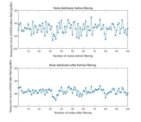
where, RSSI is the mean value of the samples; $RSSI_i$ is the filtered value at each sampling point. The RSSIs processed by the Gaussian filter are presented in Figure 1. Obviously, the Gaussian filter eliminated the excess errors induced by environmental interference and short time interference.
Figure 1. The filtered RSSIs of the Gaussian filter
2.2 Kalman filtering
Next, the measured RSSIs were further optimized by the Kalman filter, which can effectively remove mutation points and noises and realize accurate and smooth outputs.
In Kalman filtering, the state prediction equations are:
$\begin{align} & X(k|k-1)=AX(k-1|k-1)+BU(k) \\ & P(k|k-1)=AP(k-1|k-1){{A}^{T}}+Q. \\\end{align}$ (5)
The state update equations are:
$\begin{align} & X(k|k)=X(k|k-1)+Kg(k)(Z(k)-HX(k|k-1)) \\ & Kg(k)=P(k|k-1){{H}^{T}}/(HP(k|k-1){{H}^{T}}+R) \\ & P(k|k)=(I-Kg(k)H)P(k|k-1). \\\end{align}$ (6)
where, X(k|k-1) and X(k-1|k-1) are the predicted values of the current and previous states, respectively; A and B are system parameters;U(k) is current state of the control volume (default value: 0); P(k|k-1) and P(k-1|k-1) are the covariances of X(k|k-1) and X(k-1|k-1), respectively; Q is system noise. Z(k) is the measured moment for k; H is the parameters of the measurement system; Kg(k) is the Kalman filter gain; R is the measurement noise; P(k|k) is the update value of the current state; I is the unit matrix (the value is 1 for single model and measurement).
The error distribution of the RSSIs after Kalman filtering is displayed in Figure 2 below. It can be seen that the Kalman filter smoothed the outputted sample values to some extent
Figure 2. The error distribution of the RSSIs after Kalman filtering
The TSE is applicable to all kinds of channel environments. The method enjoys a low complexity and converges rapidly under proper initial values. Here, the initial positions are estimated by the weighted centroid algorithm as the initial values for the TSE. Focusing on node connectivity, the algorithm achieves a low complexity and a light computing load. In this algorithm, the unknown node receives information from all anchor nodes within its communication scope, and all these anchor nodes are considered as weighted geometric centroids. The formula of the weighted centroid algorithm can be expressed as:
$\left( {{x}_{0}},{{y}_{0}} \right)=\left( {\left( \sum{{{{x}_{i}}}/{{{R}_{i}}}\;} \right)}/{\left( \sum{{1}/{{{R}_{i}}}\;} \right),\,\left( {\left( \sum{{{{y}_{i}}}/{{{R}_{i}}}\;} \right)}/{\sum{{1}/{{{R}_{i}}}\;}}\; \right)}\; \right)\,$ (7)
The accuracy of centroid positioning relies heavily on the density and distribution of anchor nodes [13-15]. The positioning is very accurate when the nodes are dense and uniformly distributed. Otherwise, the accuracy will decrease rapidly.
During transmission, electromagnetic wave signals may be subjected to multipath interference or obstruction. In this case, the signal strength received at the same position varies from time to time [16-18]. The reliability of the measured RSSIs should be enhanced before indoor positioning. In this paper, an indoor positioning algorithm is designed with the following steps. First, the RSSI threshold is determined according to the simulation of the test environment. Second, the measured values are compared against the threshold to remove the excess errors and retain the average of the proper values. Last, the TSE is introduced to obtain the distance by equation (3).
The TSE [4], as an iterative recursive algorithm, requires accurate initial estimation of node positions to achieve fast convergence and good real-time performance. The initial positions were estimated as follows:
To begin with, the RSSIs $r_i=√((x_i-x)^2+(y_i-y)^2 )$ of an unknown node to each anchor node were measured. Then, the unknown node-anchor node distances $R_i$,i=1,2,…,N were computed as $R_i$=$r_i$+$ε_i$, where $ε_i$ is error (mean value: 0), i.e. a normal random variable of mean square error $δ^2$. In this way, the function $f_i (x,y)=√((x_i-x)^2+(y_i-y)^2 )$ is close to the initial estimate position, laying a good basis ($x_0$, $y_0$) for the TSE. After ignoring the second-order partial derivatives, the matrix representation can be obtained as:
$h\text{=}G\delta \text{+}\varepsilon $ (8)
where,
$h=\left[ \begin{matrix} -{{R}_{1}}+\sqrt{{{({{x}_{1}}+{{x}_{0}})}^{2}}+{{({{y}_{1}}-{{y}_{0}})}^{2}}} \\ -{{R}_{2}}+\sqrt{{{({{x}_{2}}+{{x}_{0}})}^{2}}+{{({{y}_{2}}-{{y}_{0}})}^{2}}} \\ \vdots \\ -{{R}_{N}}+\sqrt{{{({{x}_{N}}+{{x}_{0}})}^{2}}+{{({{y}_{N}}-{{y}_{0}})}^{2}}} \\\end{matrix} \right]$,
$A=\overline{RSSI}-\overline{n\rho }$,
$\delta \text{=}\left[ \begin{matrix} \Delta x \\ \Delta y \\\end{matrix} \right]$,
$\left( {{x}_{k}},{{y}_{k}} \right)k=1,2,\ldots ,50.$.
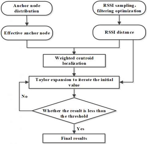
Using the weighted least squares (WLS) algorithm, the least squares estimation solutions can be derived from equation (8) as $δ={(G^T G)}^{-1} G^T h$. Then, the iterative process was initiated to determine whether |Δx|+|Δy| is less than the threshold (0.01). The estimated position was corrected iteratively until it satisfies the threshold. The iterated frequency distribution is shown in Figure 3. It can be seen that the estimated positions were stable and convergent and eventually satisfied the threshold. The last updated position was taken as the final position and compared with the actual position to obtain the positioning accuracy. The flow of the TSE algorithm is explained in Figure 4.
Figure 3. Iterated frequency distribution of the TSE
Figure 4. The flow of the TSE algorithm
The above TSE algorithm can carry out TSE at the given initial values, and correct the estimated position of the unknown node by the mean distance between the unknown node and each anchor node. This design does not consider the impact of the measured distance between the unknown node and the anchor node on Δx and Δy. In this case, the positioning error will increase significantly with the growth in the measured distance, resulting in a sharp decline in the positioning accuracy.
To solve the problem, the said measured distance was taken into account to locate the unknown node. As shown in equation (8), the weighted matrix h consists of measuring errors. According to the propagation law of radio signals, the positioning error is positively correlated with the measured distance of RSSI positioning. This correlation can be employed to reduce the impacts of excessively large or small measured distance on positioning accuracy. Specifically, the Taylor series can be improved as:
$Qh=G\delta $ (9)
where, Q is a positive definite diagonal matrix, in which the non-zero element in each row correspond to the element in the weighted matrix h. The matrix offsets the position change effect with the various elements in h, and calculates the amount of position correction of Δx and Δy according to the measured distances to the anchor nodes. Here, the Q is designed according to the calculated distances and RSSI positioning features:
$Q=\frac{1}{\left( N-1 \right)T}\left( \begin{matrix} T-{{d}_{1}}^{2} & 0 & 0 \\ 0 & \ddots & 0 \\ 0 & 0 & T-{{d}_{n}}^{2} \\\end{matrix} \right)$ (10)
where, $T=∑_{i=1}^Nd_i^2$; N is the total number of anchor node; $d_i$ is the measured distance from the unknown node to the i-th anchor node. Finally, the initial positions of the unknown node were substituted into the improved Taylor series for expansion.
The proposed method was verified through a simulation in a fixed area. The sending node was placed at a fixed position. Then, measuring points (i =1,2..., 100) were set up from the receiving node 20m away from the sending node to the fixed position at an interval of 0.2m. A total of 50 RSSIs were measured at these points, and averaged. Finally, a set of measured values were obtained from each measuring point. The measured RSSIs at each point correspond to the measured values at that distance. The 100 sets of data were plotted into a 2D coordinate system (Figure 5). Obviously, the RSSIs measured within 14m decreased gradually with the increase of the sender-receiver distance. Thus, 14m was taken as the detection range.
Figure 5. The 2D coordinates of the 100 sets of data
The radio signals propagate differently in different environments. Before simulation, the parameters A and n of the RSSI positioning model should be optimized to suit the specific environment. Using the first 70 sets of measured data $(RSSI_i,d_i )$, i=1, 2,..., 70, the A and n were calculated by linear regression analysis, and substituted into the model for further use. The optimized curve of the model demonstrates the good fitting effect of the linear regression. The linear regression can be expressed as:
$ρ_i=-10lgd_i$,i=1,2,…,70,
$n=∑_{i=1}^{70}(ρ_i -¯ρ)RSSI_i/∑_{i=1}^{70}(ρ_i -¯ρ)^2, A=¯RSSI-¯nρ$,
where, $¯RSSI=1/70 ∑_{i=1}^{70}RSSI_i$ and $¯ρ=1/70 ∑_{i=1}^{70}ρ_i$
To provide a reference for WSN positioning, several anchor nodes were randomly deployed in an area of 100*100 (m2). In other words, the positions of these nodes were randomly generated and known. The positioning accuracy was not evaluated by the deviation of the predicted position of an unknown node to the measured position. Instead, 50 unknown nodes were selected, and the positioning error of each of them was determined. Then, the mean positioning error was calculated on this basis. The actual position of each unknown node, estimated position of each unknown node and mean positioning error are respectively denoted as $(x_k,y_k)$,k=1,2,…,50, $(x ̄_k,y ̄_k )$, k=1,2,…,50 and $RMSE=1/50 ∑_{k=1}^{50}√((x_k-x ̄_k )^2-(y_k-y ̄_k )^2 )$.
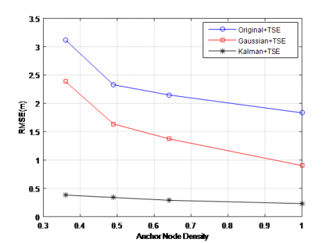
First, the RSSI positioning was carried out with different filters and the TSE in the simulation environment. The results are shown in Figure 6. It can be seen that the Gaussian filter eliminated the excess errors induced by the environmental interference and removed many of the interference resulted from short-time RSSI measurement in the volatile situation. Meanwhile, the Kalman filter smoothed the sampling value. The indoor positioning algorithm outperformed the original algorithm, after coupling Gaussian filtering, and achieved the best performance, after coupling the Kalman filtering. As shown in the figure, the proposed method achieved a no-greater-than 0.5m positioning error, whichever the anchor node density.
Figure 6. RMSEs of RSSI positioning with different filters and the TSE
Figure 7. RMSEs of RSSI positioning with different filters and the improved TSE
Second, the RSSI positioning was carried out with different filters and the improved TSE in the simulation environment. The results in Figure 7 show that the improved TSE helped improve the positioning accuracy to various degrees under different filters.
This paper mainly explores the filter optimization of RSSI positioning and proposes a correction matrix of the TSE algorithm. First, the RSSI measurement was improved by Gaussian filtering and Kalman filtering. Then, the initial position was iteratively obtained by the weighted centroid algorithm, whose weight was computed by the optimized RSSI measuring distance, and a correction matrix was developed to improve the Taylor series expansion (TSE). The simulation results show the two filtering methods, especially the Kalman filter, can effectively reduce the RSSI measurement errors and improve positioning accuracy of unknown nodes, and the correction matrix of the TSE algorithm can further improve the positioning accuracy. In addition, the positioning accuracy of our method increases with the density of anchor nodes.
This work was supported by 2017 annual “Outstanding Young Teacher Training Program” project of North China University of Technology (No.: XN019009). Scientific Research Project of Beijing Educational Committee (No.: KM201710009004). 2018 Science and technology activities project for college students of North China University of Technology (No.: 110051360007). Research project on teaching reform and curriculum construction of North China University of Technology (No.: 18XN009-011). 2019 Beijing university student scientific research and entrepreneurship action plan project (No.: 218051360019XN004). 2019 Education and teaching reform general project of North China University of Technology.
[1] Zhou HY, Yu J. (2014). Research on distance measurement based on RSSI in wireless sensor networks. Electronic Measurement Technology 37(1): 89-91.
[2] Chen L, Pang L, Zhou B, Zhang J, Liu Z, Luo Q, Sun L. (2015). RLAN: Range-free localisation based on anisotropy of nodes for WSNs. Electronics Letters 51(24): 2066-2068. https://doi.org/10.1049/el.2015.2554
[3] Zhou EL, Wang GL. (2014). Research of indoor location based on RSSI ranging. Journal of Chongqing University of Technology (Natural Science) 28(9): 98-101.
[4] Li Z, Huang JS. (2016). WiFi positioning using robust filtering with RSSI. Geomatics and Information Science of Wuhan University 41(3): 361-366.
[5] Rasool I, Salman N, Kemp A. (2012). RSSI-based positioning in unknown path-loss model for WSN. Sensor Signal Processing for Defence (SSPD 2012) 1- 5. https://doi.org/10.1049/ic.2012.0112
[6] Wan GF, Zhong J, Yang CH. (2012). Improved algorithm of ranging and locating based on RSSI. Application Research of Computers 29(11): 4156-4158.
[7] Thaljaoui A, Val T, Nasri N, Brulin D. (2015). BLE localization using RSSI measurements and iRingLA. 2015 IEEE International Conference on Industrial Technology (ICIT), pp. 2178-2183. https://doi.org/10.1109/ICIT.2015.7125418
[8] Jin R, Che Z, Xu H, Wang Z, Wang L. (2015). An RSSI-based localization algorithm for outliers suppression in wireless sensor networks. Wireless Networks 21(8): 2561-2569. https://doi.org/10.1007/s11276-015-0936-x
[9] Zhang Z, Ra ZX. (2013). Some methods of RSSI filtering in wireless sensor networks. Modern Electronics Technique 36(20): 4-6.
[10] Tang T, Hui HH. (2013). Gaussian curve fitting solution based on Matlab. Computer & Digital Engineering 41(8): 1262-1263.
[11] Alraih S, Alhammadi A, Shayea I, AI-Samman AM. (2017). Improving accuracy in indoor localization system using fingerprinting technique. 2017 International Conference on Information and Communication Technology Convergence (ICTC), pp. 274-277. https://doi.org/10.1109/ICTC.2017.8190985
[12] Chen C, Chen Y, Han Y, Lai HQ, Zhang F, Liu KJR. (2016). Achieving centimeter-accuracy indoor localization on WiFi platforms: A multi-antenna approach. IEEE Internet of Things Journal 4(1): 122-134. https://doi.org/10.1109/JIOT.2016.2628713
[13] Zhuang Y, Kang YH, Huang L, Fang ZX. (2018). A geocoding framework for indoor navigation based on the QR code. 2018 Ubiquitous Positioning, Indoor Navigation and Location-Based Services (UPINLBS), pp. 1-4. https://doi.org/10.1109/UPINLBS.2018.8559741
[14] Molia B, Olivares E, Palau CE, Esteve M. (2018). A multimodal fingerprint-based indoor positioning system for airports. IEEE Access 6: 10092-10106. https://doi.org/10.1109/ACCESS.2018.2798918
[15] Tao Y, Zhao L. (2018). A novel system for WiFi radio map automatic adaptation and indoor positioning. IEEE Transactions on Vehicular Technology 67(11): 10683-10692. https://doi.org/10.1109/TVT.2018.2867065
[16] Sun W, Xue M, Yu HS, Tang HW, Lin A. (2018). Augmentation of fingerprints for indoor WiFi localization based on gaussian process regression. IEEE Transactions on Vehicular Technology 67(11): 10896-10905. https://doi.org/10.1109/TVT.2018.2870160
[17] Tian XH, Li WX, Yang YC, Zhang ZH, Wang XB. (2008). Optimization of fingerprints reporting strategy for WLAN indoor localization. IEEE Transactions on Mobile Computing 17(2): 390-403. https://doi.org/10.1109/TMC.2017.2715820
[18] Sou SL, Lin WH, Lan KC, Lin CS. (2019). Indoor location learning over wireless fingerprinting system with particle Markov chain model. IEEE Access 7: 8713-8725. https://doi.org/10.1109/ACCESS.2019.2890850