Ravi Shankar* | Indrajeet Kumar| Ritesh Kumar Mishra
© 2019 IIETA. This article is published by IIETA and is licensed under the CC BY 4.0 license (http://creativecommons.org/licenses/by/4.0/).
OPEN ACCESS
The objective of this study is to examine the outage probability (OP) performance of the multiple-input multiple-output (MIMO) cooperative communication system over Nakagami-m fading channel conditions. Source node transmits orthogonal space time block code (OSTBC) codeword to the relay & destination node and maximal ratio combiner (MRC) is used for the decoding purpose at the destination node. A mathematical framework is developed for the analysis of diversity order (DO) of the system. The closed form expression of OP is derived in terms of confluent hypergeometric function of two variables considering perfect channel state information (CSI). The Simulation results verified the accuracy of the derived analytical results. Furthermore, the results shown that the distances between the nodes significantly affect the OP performance.
cooperative communication, outage probability, pairwise error probability, channel state information, convex optimization
Wireless channel is broadcast in nature i.e., transmission of data in the air where everyone can receive. This nature can be exploited to achieve cooperative diversity. Using Cooperative communication [1], other users can cooperate with the source in forwarding the data to the destination node. The main advantage of the cooperative communication is if direct source-to-destination (SD) channel is in deep fade, the destination can still receive the source signal through relay. Relay assisted cooperation is the first step towards the 5th generation (5G) wireless system, which is expected to offer up to 20Gbps in the downlink (D/L) and 10Gbps in uplink (U/L) wireless communication [2]. Numerous relaying schemes have been proposed in the existing literatures such as amplify-and-forward (AF) [3-5], decode-and-forward (DF) [6] and selective decode and forward (S-DF) [7-12]. However, the works [3-6] suffer from several significant drawbacks. Firstly, the system performance is limited due to the noise amplification problem because of the consideration of the AF relaying protocol. Secondly, in case of DF protocol, the relay node may forward erroneous signal to the destination node. To overcome this problem S-DF is proposed. In case of S-DF relaying protocol, relay only forwards correctly decoded signal to the destination node. In the work [13], the authors investigated the multiple hop multiple phase S-DF relaying protocol considering perfect CSI conditions. Asymptotic tight expression of symbol error rate (SER) is derived employing quadrature phase shift keying (QPSK) modulation schemes and shown to be tight at high signal to noise ratio (SNR) regimes. Results show that end-to-end system performance improves with optimal source-relay power allocation factors. In [14], the authors investigate the OP performance of a single input single output (SISO) cooperative communication system over Nakagami-m fading channel conditions. In [15], the authors present the novel framework for optimizing and investigating the OP performance of a MIMO AF cooperative communication network, where K relays, each with finite cache capacity, are deployed to assist the transmission from a base station equipped with R antennas to the destination. The authors present the best relay selection criterion to choose the best relay, which maximizes the received SNR at the receiving terminal. For this criterion, we derive asymptotic and exact theoretical expressions for the system OP over independent and identically distributed (i.i.d.) Nakagami-m fading channel conditions. In the works [16-17], the authors investigate the D/L full duplex non-orthogonal multiple access (NOMA) cooperative communication network model and selective DF technique over Nakagami-m fading channel with imperfect CSI. This work assumes that the destination and the source node have fixed power, whereas relay nodes have constrained energies and should harvest radio frequency (RF) energy from the source for operation power. However, to the best of our knowledge, there has been no work to derive the exact OP of the destination SNR in MIMO OSTBC S-DF relaying network over Nakagami-m fading channel conditions.
We conclude the following novel contributions from this paper:
(1). The closed form OP expressions are derived for MIMO OSTBC S-DF relaying network over Nakagami-m fading channel, with perfect CSI.
(2). Further, a framework is developed for deriving the DO for MIMO OSTBC S-DF relaying network.
The rest of the paper is organized as follows; MIMO OSTBC S-DF system model is given in section 2. OP performance and DO analysis have been given in Section 3. In section 4, simulation results are given and finally in section 5 paper conclusions are given.
Consider MIMO OSTBC S-DF relaying network in which the source, relay and destination nodes are equipped $M_S$, $M_R$ and $M_D$ number of antennas, respectively [13]. Spatially uncorrelated flat fading Nakagami-m fading channel is considered, and the fading links are assumed to be independent and identically distributed with each other. Since the source and relay nodes are employed by same OSTBC, we take $M_S=M_R=M$ [9]. The signal transmission is divided into two phases, broadcast phase and relaying phase. During the broadcast phase, the source node transmits the MIMO OSTBC codeword $B_S∈C^{M*T_S}$ to relay and destination, respectively. Where $T_s$ represents the number of time slots. The received code-word's at the destination node, $Y_{SD}∈C^{M_D×T_S}$ and at the relay node, $Y_{SR}∈C^{M×T_S}$ corresponding to the MIMO OSTBC code-word transmission from the source node can be written as [12],
${{Y}_{SD}}=\sqrt{{{P}_{S}}/M{{R}_{C}}}{{H}_{SD}}{{B}_{S}}+{{Z}_{SD}},$ (1)
${{Y}_{SR}}=\sqrt{{{P}_{S}}/M{{R}_{C}}}{{H}_{SR}}{{B}_{S}}+{{Z}_{SR}}.$ (2)
where $P_s$ and $R_c$ denote the available power at the source node and coding rate, respectively. The terms of the SD $H_{SD}∈C^{M_D×M}$ and source-to-relay (SR) $H_{SR}∈C^{M×M}$ channel matrices are independent with each other, distributed as Nakagami-m random variables (RVs) with a fading severity or shape parameter, $m_i≥0.50; i∈{SD,SR}$ and controlling spreads $δ_{SD}^2$ and $δ_{SD}^2$ respectively [19]. The channel fades for different links are assumed to be statistically independent. This is a reasonable assumption as the relays are usually spatially well separated. In the relaying phase, relay node re-transmits only successfully decoded
Figure 1. MIMO-OSTBC S-DF cooperative communication
Signal to the destination node, otherwise, it will remain in the idle state. The received symbol blocks at the destination node $Y_{SD}∈C^{M_D×T_S}$ corresponding to transmission from relay node can be written as [13],
${{Y}_{RD}}=\sqrt{{{P}_{R}}/M{{R}_{C}}}{{H}_{RD}}{{B}_{S}}+{{Z}_{RD}}.$ (3)
where $P_R$ denotes the power transmitted from the relay node. The relay-to-destination (RD) channel matrix $H_{RD}∈C^{M_D×M}$ is comprised of terms, which are independent with each other, distributed as Nakagami-m RVs with a fading severity or shape parameter, $m_RD≥0.50$ and controlling spread $δ_{RD}^2$. The channel noise matrices $Z_RD$, $Z_SR$ and $Z_SD$ in (3), (2) and (1), respectively, are zero mean circular shift complex gaussian (ZMCSCG) RVs with variance $N_0$, respectively. Since the OSTBC based MIMO transmission orthogonalizes and converts the MIMO fading channel into scalar channels. The instantaneous SNR at the receiving terminal (destination node) is given as,
${{\gamma }_{D}}=\frac{{{c}_{O}}{{P}_{S}}}{{{R}_{C}}M{{N}_{0}}}\left\| {{H}_{SD}} \right\|_{F}^{2}+\,{{A}_{R}}\frac{{{c}_{1}}{{P}_{R}}}{RM{{N}_{0}}}\left\| {{H}_{RD}} \right\|_{F}^{2}.$ (4)
Here, $A_r$ represents the state of the relay node, is given as,
${{A}_{R}}=\left\{ \begin{matrix} 0\,\,\,\,if\,{{\gamma }^{R}}\,\,<\gamma _{T}^{R} \\ 1\,\,\,\,\,if\,{{\gamma }^{R}}\,\,\ge \,\gamma _{T}^{R}\, \\\end{matrix} \right..$ (5)
where $γ_T^R$ and $γ^R$ denotes the threshold SNR and the instantaneous SNR at the relay node, respectively. The $γ^R$ cab be written as,
${{\gamma }^{R}}=\frac{{{c}_{2}}{{P}_{S}}}{{{R}_{C}}M{{N}_{0}}}\left\| {{H}_{SR}} \right\|_{F}^{2}.$ (6)
where $c_1$, $c_1$ and $c_0$ denote the power dependent power transfer factors for the source-relay, relay-destination and source-destination channels, respectively. The OP $P_{γ_T^D}^OP$ can be written as,
$\begin{align} & P_{\gamma _{T}^{D}}^{OUTAGE}= \\ & \,\,\,\,\,\,\,\,\,\Pr \left\{ {{\gamma }^{D}}\left| _{{{A}_{r}}=0} \right.\le \gamma _{T}^{D} \right\}\Pr \left\{ {{A}_{r}}=0 \right\}+\,\Pr \left\{ {{\gamma }^{D}}\left| _{{{A}_{r}}=1} \right.\le \gamma _{T}^{D} \right\}\Pr \left\{ {{A}_{r}}=1 \right\}. \\\end{align}$ (7)
where $γ_T^D$ and $Pr{.}$ denote the threshold SNR at the destination node and probability operator, respectively. In this work, it is assumed that the source and relay node consume equal power, i.e., equal power allocation, so we can take, $P_S≤P/2$ and $P_R≤P/2$, where P denotes the total available power budget. Also, it has been considered that the relay and source node do not have the knowledge of RD and SD channel gains, respectively. Now, it obvious that the relay and source transmit with their maximum powers. Utilizing these transmit powers, the following notations,
$P_0'≜c_0 ρ/2,P_1'≜c_1 ρ/2,P_2'≜c_1 ρ/2$,
where
$\rho =P/R{{N}_{0}}M,$ (8)
and assuming $γ_T^D=γ_T^R=γ_T$ for simplicity purpose, OP expression given in (7) can be written as,
$\begin{align} & P_{{{\gamma }_{T}}}^{OUTAGE}= \\ & \Pr \left\{ P_{0}^{'}\left\| {{H}_{SD}} \right\|_{F}^{2}\le {{\gamma }_{T}} \right\}\Pr \left\{ P_{2}^{'}\left\| {{H}_{SR}} \right\|_{F}^{2}<{{\gamma }_{T}} \right\} \\ & +\,\Pr \left\{ P_{0}^{'}\left\| {{H}_{SD}} \right\|_{F}^{2}+P_{1}^{'}\left\| {{H}_{RD}} \right\|_{F}^{2}\le {{\gamma }_{T}} \right\}\Pr \left\{ P_{2}^{'}\left\| {{H}_{SR}} \right\|_{F}^{2}\ge {{\gamma }_{T}} \right\}. \\\end{align}$ (9)
We assume that RD distance is smaller than the SD distance. Note that $c_0$ and $c_1$ impact the link-budget and the normalized fading comes on top of this. Therefore, we can write $c_0≤c_1$ which implies that $P_0'≤P_1'$ (see (8) above). This scenario is necessary for further mathematical development in section 3.
3.1 OP analysis
Using the notations
$a\triangleq {{{P}'}_{0}}\left\| {{H}_{SD}} \right\|_{F}^{2},b\triangleq {{{P}'}_{1}}\left\| {{H}_{RD}} \right\|_{F}^{2},g\triangleq {{{P}'}_{2}}\left\| {{H}_{SR}} \right\|_{F}^{2},$ (10)
and $h≜a+b$, the OP expression given in (9) can be written a
$P_{{{\gamma }_{T}}}^{OUTAGE}=\Pr \left\{ a\le {{\gamma }_{T}} \right\}\Pr \left\{ g<{{\gamma }_{T}} \right\}+\,\Pr \left\{ h\le {{\gamma }_{T}} \right\}\Pr \left\{ g\ge {{\gamma }_{T}} \right\}.$ (11)
It is noted that a, b and g are Chi-square distributed RV with the degree of freedom $2M_R M_D m_SD$, $2M_R M_D m_RD$ and $2M_S M_R m_SR$, respectively. The probability density expression (PDF) of Chi-square distributed RV can be expressed as,
${{f}_A}\left( a \right)=\frac{{{a}^{{{M}_{R}}{{M}_{D}}{{m}_{SD}}-1}}}{{{\left( 2P_{0}^{'} \right)}^{^{{{M}_{R}}{{M}_{D}}{{m}_{SD}}}}}\Gamma \left( {{M}_{R}}{{M}_{D}}{{m}_{SD}} \right)}{{e}^{-\frac{a}{2P_{0}^{'}}}}.$ (12)
Applying the similar procedure, we can express the PDF of Chi-square distributed RV b and g respectively in similar form as given in (12).
By performing some mathematical manipulations, it can be shown that,
$\begin{align} & \Pr \left\{ a\le {{\gamma }_{T}} \right\}=\frac{\gamma \left( {{M}_{R}}{{M}_{D}}{{m}_{SD}},\frac{{{\gamma }_{T}}}{2P_{0}^{'}} \right)}{\Gamma \left( {{M}_{R}}{{M}_{D}}{{m}_{SD}} \right)}, \\ & \Pr \left\{ g\ge {{\gamma }_{T}} \right\}=\frac{\Gamma \left( M_{R}^{2}{{m}_{SR}},\frac{{{\gamma }_{T}}}{2P_{2}^{'}} \right)}{\Gamma \left( M_{R}^{2}{{m}_{SR}} \right)}. \\\end{align}$ (13)
where $Γ(.)$, $Γ(.,.)$ and $Γ(.)$ denote the Gamma function, upper incomplete Gamma function and lower incomplete Gamma function, respectively [18].
3.2 Derivation for the PDF of h
The PDF of h can be found out by using the concept of characteristics function (CF). The CF of h can be expressed as the product of CF of a and b, can be expressed as,
${{\Upsilon }_A}\left( \alpha \right)=\int_{0}^{\infty }{{{f}_A}\left( a \right){{e}^{ja\alpha }}}da.$ (14)
Using (12) into (14) and using [(3.381.4) [18]], $ϒ_Α (α)$ can be written as,
${{\Upsilon }_A}\left( \alpha \right)={{(1-i2{{{P}'}_{0}}\alpha )}^{-{{M}_{R}}{{M}_{D}}{{m}_{SD}}}}.$ (15)
Following the similar procedure, the CF of b can be expressed as,
${{\Upsilon }_{B}}\left( \alpha \right)={{(1-i2{{{P}'}_{1}}\alpha )}^{-{{M}_{R}}{{M}_{D}}{{m}_{RD}}}}.$ (16)
The CF of h can be expressed as,
$\begin{align} & {{\Upsilon }_{H}}\left( \alpha \right)={{\Upsilon }_{B}}\left( \alpha \right)\times {{\Upsilon }_A}\left( \alpha \right) \\ & \,\,\,\,\,\,\,\,\,\,\,\,\,\,\,={{(1-i2{{{{P}'}}_{1}}\alpha )}^{-{{M}_{R}}{{M}_{D}}{{m}_{RD}}}}\times {{(1-i2{{{{P}'}}_{0}}\alpha )}^{-{{M}_{R}}{{M}_{D}}{{m}_{SD}}}}. \\\end{align}$ (17)
The PDF of h can be expressed as,
${{f}_{H}}\left( h \right)=\frac{1}{2\pi }\int_{0}^{\infty }{{{\Upsilon }_{H}}\left( \alpha \right){{e}^{-jh\alpha }}}d\alpha .$ (18)
Substituting the expression of $ϒ_H (α)$ into (18) and utilizing [(3.384.7) [18]], $f_H (h)$ can be expressed as,
$\begin{align} & {{f}_{H}}\left( h \right)= \\ & \frac{{{h}^{({{M}_{R}}{{M}_{D}}{{m}_{SD}}+{{M}_{R}}{{M}_{D}}{{m}_{RD}}-1)}}{{e}^{-\,\frac{h}{2P_{0}^{'}}}}}{{{(2P_{0}^{'})}^{{{M}_{R}}{{M}_{D}}{{m}_{SD}}}}{{(2P_{1}^{'})}^{{{M}_{R}}{{M}_{D}}{{m}_{RD}}}}\Gamma \left( {{M}_{R}}{{M}_{D}}{{m}_{SD}}+{{M}_{R}}{{M}_{D}}{{m}_{RD}} \right)}\times \\ & \underbrace{{}_{1}{{F}_{1}}\left\{ {{M}_{R}}{{M}_{D}}{{m}_{SD}};{{M}_{R}}{{M}_{D}}{{m}_{SD}}+{{M}_{R}}{{M}_{D}}{{m}_{RD}};\left( \frac{1}{2P_{0}^{'}}-\frac{1}{2P_{1}^{'}} \right)h \right\}}_{L\left( h \right)}. \\\end{align}$ (19)
where $_1F_1 (.)$ represents the single variable’s confluent hypergeometric function [(9.210) [18]].
Using [(9.211.2) [18]], we get,
$\begin{align} & L\left( h \right)= \\ & \frac{1}{\Xi \left( {{M}_{R}}{{M}_{D}}{{m}_{SD}},{{M}_{R}}{{M}_{D}}{{m}_{RD}} \right)}\int_{0}^{1}{{{e}^{\left( \frac{1}{2P_{0}^{'}}-\frac{1}{2P_{1}^{'}} \right)ht}}}{{t}^{{{M}_{R}}{{M}_{D}}{{m}_{SD}}-1}}{{\left( 1-t \right)}^{{{M}_{R}}{{M}_{D}}{{m}_{RD}}-1}}dt. \\\end{align}$ (20)
where Ξ($M_R M_D m_SD,M_R M_D m_RD$)denotes the Beta function [18], defined as,
$\Xi \left( {{M}_{R}}{{M}_{D}}{{m}_{SD}},{{M}_{R}}{{M}_{D}}{{m}_{RD}} \right)=\frac{\left| \!{\overline {\, {{M}_{R}}{{M}_{D}}{{m}_{SD}} \,}} \right. \times \left| \!{\overline {\, {{M}_{R}}{{M}_{D}}{{m}_{SD}} \,}} \right. }{\left| \!{\overline {\, {{M}_{R}}{{M}_{D}}{{m}_{SD}}+{{M}_{R}}{{M}_{D}}{{m}_{RD}} \,}} \right. }.$ (21)
By using the notation
$\begin{align} & {{E}_{K}}\triangleq \\ & \frac{1}{{{(2P_{0}^{'})}^{{{M}_{R}}{{M}_{D}}{{m}_{SD}}}}{{(2P_{1}^{'})}^{{{M}_{R}}{{M}_{D}}{{m}_{RD}}}}\Gamma \left( {{M}_{R}}{{M}_{D}}{{m}_{SD}}+{{M}_{R}}{{M}_{D}}{{m}_{RD}} \right)\Xi \left( {{M}_{R}}{{M}_{D}}{{m}_{SD}},{{M}_{R}}{{M}_{D}}{{m}_{RD}} \right)} \\\end{align}$ (22)
and some mathematical arrangements and manipulations, we get,
$\Pr \left\{ h\le {{\gamma }_{T}} \right\}=1-{E_K}\int_{0}^{1}{{{P}_{1}}}{{t}^{{{M}_{R}}{{M}_{D}}{{m}_{SD}}-1}}{{\left( 1-t \right)}^{{{M}_{R}}{{M}_{D}}{{m}_{RD}}-1}}dt,$ (23)
where $P_1$ is expressed as,
${{P}_{1}}=\int\limits_{{{\gamma }_{T}}}^{\infty }{{{e}^{-\frac{1}{2P_{0}^{'}}}}^{\left( 1-\left( 1-\frac{P_{0}^{'}}{P_{1}^{'}} \right)t \right)h}{{h}^{{{M}_{R}}{{M}_{D}}{{m}_{SD}}+{{M}_{R}}{{M}_{D}}{{m}_{RD}}-1}}}dh.$ (24)
Using [(3.381.3) [18]], (24) can be expressed as,
${{P}_{1}}={{\left( s \right)}^{-{{M}_{R}}{{M}_{D}}{{m}_{SD}}+{{M}_{R}}{{M}_{D}}{{m}_{RD}}}}\Gamma \left( {{M}_{R}}{{M}_{D}}{{m}_{SD}}+{{M}_{R}}{{M}_{D}}{{m}_{RD}},\,s{{\gamma }_{T}} \right)$ (25)
where for simplicity, s is defined as,
$s=\frac{1}{2P_{0}^{'}}\left( 1-\left( 1-\frac{P_{0}^{'}}{P_{1}^{'}} \right)t \right).$ (26)
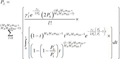
Using the series representation of $Γ(M_R M_D m_SD+M_R M_D m_RD,sγ_T )$ [(8.352.2)] and some mathematical manipulations, we get,
(27)
In the integral given above, s is a function of t. Substituting the value of s given in (26) into (27), the mathematical manipulation leads to,
(28)
Utilizing [(3.385) [18]], we get the closed-form expression ofP_2in the form of confluent hypergeometric function $Φ_1 {A_11,B_11,C_11,a,b}$ of the variable a and b [(9.261.1) [18]]. Utilizing (21), (8) and $P_2$ in terms of $Φ_1 ()$, (27) can be expressed as,
(29)
The series of $Φ_1 (.)$ can be efficiently evaluated by applying the approximation $(1-c_0/c_1 )<1$. Substituting (13) into (11), the OP can be expressed as,
$\begin{align} & P_{{{\gamma }_{T}}}^{OUTAGE}= \\ & \frac{\gamma \left( {{M}_{R}}{{M}_{D}}{{m}_{SD}},\,\,\frac{{{\gamma }_{T}}}{\rho {{c}_{0}}} \right)}{\Gamma \left( {{M}_{R}}{{M}_{D}}{{m}_{SD}} \right)}\frac{\gamma \left( M_{R}^{2}{{m}_{SR}},\frac{{{\gamma }_{T}}}{\rho {{c}_{2}}} \right)}{\Gamma \left( M_{R}^{2}{{m}_{SR}} \right)}+\,\Pr \left\{ h\le {{\gamma }_{T}} \right\}\frac{\Gamma \left( M_{R}^{2}{{m}_{SR}},\frac{{{\gamma }_{T}}}{\rho {{c}_{2}}} \right)}{\Gamma \left( M_{R}^{2}{{m}_{SR}} \right)}. \\\end{align}$ (30)
3.3 3DO Analysis
In case of high SNR, i.e., $ρ→∞$, $P_{γ_T}^{OUTAGE}$ tends to 0. It can easily show by using $P_2$ for $Φ_1 ()$, utilizing [(8.352) [18]], [(3.197.3) [18]], [(8.352.1) [18]] & [(9.131) [18]]. The opposite scenario that $P_{γ_T}^{OUTAGE}$ tends to 1 as $ρ→0$ can be easily confirm for (30). While checking the high SNR scenario, it can be seen that the negative exponent of $ρ$ does not depend on $c_1$ and $c_0$. Thus, for simplicity purpose, we take $c_1=c_0$ for which $Φ_1 ()$ in (29) tends to 1. Utilizing [(8.352.1) [18]] to (29), (30) can be simplified as,
$P_{γ_T}^{OUTAGE}=γ(M_R M_D m_{SD},γ_T/(ρc_0 ))/Γ(M_R M_D m_{SD} ) γ(M_R^2 m_{SR},γ_T/(ρc_2 ))/Γ(M_R^2 m_{SR})$
$+γ(M_R M_D m_{SD}+M_R M_D m_{RD},γ_T/(ρc_0 ))/Γ(M_R M_D m_{SD}+M_R M_D m_{RD})Γ(M_R^2 m_{SR},γ_T/(ρc_2 ))/Γ(M_R^2 m_{SR})$ .
It can be easily shown that the cooperation improves the DO of the system. For high SNR scenario the outage probability expression can be expressed as,
$\begin{align} & \frac{\gamma _{T}^{{{M}_{R}}{{M}_{D}}{{m}_{SD}}+{{M}_{R}}{{M}_{R}}{{m}_{SR}}}{{\rho }^{-{{M}_{R}}{{M}_{D}}{{m}_{SD}}-{{M}_{R}}{{M}_{R}}{{m}_{SR}}}}}{c_{0}^{{{M}_{R}}{{M}_{D}}{{m}_{SD}}}c_{2}^{{{M}_{R}}{{M}_{R}}{{m}_{SR}}}\Gamma \left( {{M}_{R}}{{M}_{D}}{{m}_{SD}} \right)\Gamma \left( {{M}_{R}}{{M}_{R}}{{m}_{SR}} \right)M_{R}^{3}{{M}_{D}}}+\, \\ & \frac{\gamma _{T}^{{{M}_{R}}{{M}_{D}}{{m}_{SD}}+{{M}_{R}}{{M}_{D}}{{m}_{RD}}}{{\rho }^{-({{M}_{R}}{{M}_{D}}{{m}_{SD}}+{{M}_{R}}{{M}_{D}}{{m}_{RD}})}}}{c_{0}^{{{M}_{R}}{{M}_{D}}{{m}_{SD}}+{{M}_{R}}{{M}_{D}}{{m}_{RD}}}\Gamma \left( {{M}_{R}}{{M}_{D}}{{m}_{SD}}+{{M}_{R}}{{M}_{D}}{{m}_{RD}} \right)({{M}_{R}}{{M}_{D}}{{m}_{SD}}+{{M}_{R}}{{M}_{D}}{{m}_{RD}})} \\ & -\,\frac{\gamma _{0}^{{{M}_{R}}{{M}_{D}}{{m}_{SD}}+{{M}_{R}}{{M}_{D}}{{m}_{RD}}+{{M}_{R}}{{M}_{R}}{{m}_{SR}}}{{\rho }^{-({{M}_{R}}{{M}_{D}}{{m}_{SD}}+{{M}_{R}}{{M}_{D}}{{m}_{RD}})-{{M}_{R}}{{M}_{R}}{{m}_{SR}}}}}{c_{0}^{{{M}_{R}}{{M}_{D}}{{m}_{SD}}+{{M}_{R}}{{M}_{D}}{{m}_{RD}}}c_{2}^{{{M}_{R}}{{M}_{R}}{{m}_{SR}}}\Gamma \left( {{M}_{R}}{{M}_{D}}{{m}_{SD}}+{{M}_{R}}{{M}_{D}}{{m}_{RD}} \right)\Gamma \left( {{M}_{R}}{{M}_{R}}{{m}_{SR}} \right)2M_{R}^{3}{{M}_{D}}} \\\end{align}$ (31)
The OP expression is dominate by the first two terms of (31). The DO becomes $M_R M_D m_{SD}$+$M_R M_R m_{SR}$ and $M_R M_D m_{SD}$+$M_R M_D m_{RD}$ for $M_D>M_R$ and $M_D≤M_R$, respectively. For special case when $A_R=1$, the asymptotic value of OP is completely described by the second term of (31) and DO expression becomes independent of the value of $M_R$ and $M_D$, for this special case DO is expressed as $M_R M_D m_{SD}+M_R M_D m_{RD}$.
Monte-Carlo (MC) simulation are given to confirm the accuracy of the theoretical OP expression given in (30). Simulation parameters are, $M_R=1$, $R_C=1$, $c_0=0.80$, $c_1=0.90$, $c_2=0.95$, $γ_T=5dB$ and $P_T=4dBw$. The Alamouti STBC codeword is used with 4-PSK modulation symbols. We consider the flat fading case and it has been assumed that the $H_SD$, $H_SR$ and $H_RD$ are constant during the two consecutives symbols. The total number of symbols transmission per iteration is $10^6$. Figure 2 compares the OP obtained via MC simulations and analytical calculation vs.ρ for cooperation system with different number of $M_D$. We have also shown the performance comparison between the non-cooperation system with the cooperation system. Plot shows that the relaying system outperforms the non-cooperative schemes. With increase in the value of $M_D$, OP performance improves. Also, it is shown that with the increasing value of ρ, the OP decreases. Simulated plots confirm the accuracy of the analytical results.
Figure 2. OP performance for various number of antennas at the destination node
In this paper, we analyzed the OP performance of the MIMO-OSTBC S-DF cooperative communication system over Nakagami-m fading channel conditions. Based on the assumption that channel estimation is error free, i.e., perfect CSI, we derived the OP of the MIMO-OSTBC S-DF cooperative communication system. The closed form expression of OP is derived in terms of confluent hypergeometric function of two variables. The Simulation results verified the accuracy of the derived analytical results. In addition, the results showed that the distance between nodes greatly influences OP performance. However, to theoretically obtain an optimal source-relay power splitting ratio based on the the OP analysis is left as a future study.
[1] Ray Liu KJ, Sadek AK, Su WF, Kwasinski A. (2009). Cooperative communications and networking. Cambridge University Press. https://doi.org/10.1017/CBO9780511754524
[2] https://www.networkworld.com/article/2941362/next-generation-5g-speeds-will-be-10-to-20 gbps.html
[3] Khattabi YM, Matalgah MM. (2018). Alamouti-OSTBC wireless cooperative networks with mobile nodes and imperfect CSI estimation. IEEE Transactions on Vehicular Technology 67(4): 3447-3456. https://doi.org/10.1109/TVT.2017.2786471
[4] Khattabi Y, Matalgah MM. (2016). A low-complexity sub-optimal decoder for OSTBC-based mobile cooperative systems. In 2016 IEEE Wireless Communications and Networking Conference, pp. 1-6. https://doi.org/10.1109/WCNC.2016.7565132
[5] Khattabi, Y, Matalgah MM. (2016). Improved error performance ZFSTD for high mobility relay-based cooperative systems. Electronics Letters 52(4): 323-325. https://doi.org/10.1049/el.2015.3239
[6] Bhatnagar MR, Hjorungnes A. (2011). ML decoder for decode-and-forward based cooperative communication system. IEEE Transactions on Wireless Communications 10(12): 4080-4090. https://doi.org/10.1109/TWC.2011.100611.101341
[7] Shankar R, Mishra RK. (2018). An investigation of S-DF cooperative communication protocol over keyhole fading channel. Physical Communication 29: 120-140. https://doi.org/10.1016/j.phycom.2018.04.027
[8] Kumar I, Sachan V, Shankar R, Mishra RK. (2018). An investigation of wireless S-DF hybrid satellite terrestrial relaying network over time selective fading channel. Traitement du Signal 35(2): 103-120. https://doi.org/10.3166/ts.35.103-120
[9] Sachan V, Kumar I, Shankar R, Mishra RK. (2018). Analysis of transmit antenna selection based selective decode forward cooperative communication protocol. Traitement du Signal 35(1): 47-60. https://doi.org/10.3166/ts.35.47-60
[10] Shankar R, Kumar I, Kumari A, Pandey KN, Mishra RK. (2017). Pairwise error probability analysis and optimal power allocation for selective decode-forward protocol over Nakagami-m fading channels. In 2017 International Conference on Algorithms, Methodology, Models and Applications in Emerging Technologies (ICAMMAET), pp. 1-6. IEEE. https://doi.org/10.1109/ICAMMAET.2017.8186700
[11] Shankar R, Pandey KN, Kumari A, Sachan V, Mishra RK. (2017). C(0) protocol based cooperative wireless communication over Nakagami-m fading channels: PEP and SER analysis at optimal power. 2017 IEEE 7th Annual Computing and Communication Workshop and Conference (CCWC), Las Vegas, pp. 1-7. https://doi.org/10.1109/CCWC.2017.7868399
[12] Shankar R, Kumar G, Sachan V, Mishra RK. (2018). An investigation of two-phase multi-relay S-DF cooperative wireless network over time-variant fading channels with incorrect CSI. Procedia Computer Science 125: 871-879. https://doi.org/10.1016/j.procs.2017.12.111
[13] Varshney N, Krishna AV, Jagannatham AK. (2015). Selective DF protocol for MIMO STBC based single/multiple relay cooperative communication: End-to-end performance and optimal power allocation. In IEEE Transactions on Communications 63(7): 2458-2474. https://doi.org/10.1109/TCOMM.2015.2436912
[14] Suraweera HA, Smith PJ, Armstrong J. (2006). Outage probability of cooperative relay networks in Nakagami-m fading channels. In IEEE Communications Letters 10(12): 834-836. https://doi.org/10.1109/LCOMM.2006.060834
[15] Fan L, Zhao N, Lei X, Chen Q, Yang N, Karagiannidis GK. (2018). Outage probability and optimal cache placement for multiple amplify-and-forward relay networks. In IEEE Transactions on Vehicular Technology 67(12): 12373-12378. https://doi.org/10.1109/TVT.2018.2872874
[16] Tan NT, Hoang TM, Nguyen BC, Dung LT. (2018). Outage analysis of downlink NOMA full-duplex relay networks with RF Energy harvesting over Nakagami-m fading channel. In International Conference on Engineering Research and Applications, pp. 477-487. https://doi.org/10.1007/978-3-030-04792-4_62
[17] Hou T, Sun X, Song Z. (2018). Outage performance for non-orthogonal multiple access with fixed power allocation over Nakagami-m fading channels. In IEEE Communications Letters 22(4): 744-747. https://doi.org/10.1109/LCOMM.2018.2799609
[18] Jeffrey A, Zwillinger D. (2007). Table of integrals, series, and products. Elsevier EBOOK ISBN:9780080471112, Hardcover ISBN: 9780123736376.
[19] Yacoub MD, Fraidenraich G, Santos Filho JCS. (2010). Nakagami-m phase-envelope joint distribution: A new model. IEEE Transactions on Vehicular Technology 59(3): 1552-1557. https://doi.org/10.1109/TVT.2010.2040641