Hui Liang| Qian Zhang* | Chang Fu| Fei Liang| Yusheng Sun
© 2019 IIETA. This article is published by IIETA and is licensed under the CC BY 4.0 license (http://creativecommons.org/licenses/by/4.0/).
OPEN ACCESS
Considering the immense value and preservation difficulty of Jun ware, this paper designs a novel digital modelling strategy that captures and simulates the shape of Jun ware as a 3D computer model. The ordinary differential equation (ODE)-based modelling technique, which is known for its high accuracy, was introduced to simulate the complex curve surface and stitch up the connection parts produced by different moulds. The ODE-based modelling was tailored to the two main groups of Jun ware: General Jun ware and Official Jun ware. The analysis show that our modelling method keeps Jun ware design simple and engaging to young craftsmen.
ordinary differential equation (ODE), shape modelling, digital modelling, Jun ware
Jun ware is a type of Chinese pottery, one of the Five Great Kilns of Song dynasty ceramics. From material selection to moulding, the ware is endowed with rich cultural and artistic value in very production step. The classic works boast enormous cultural and economic value nowadays. In 2016, Christie’s auctioned several Jun wares at fancy prices in New York, including USD 52,500 for a small blue bowl, USD 112,500 for a blue plate splashed with purple, and USD 389,000 for a round No.3 jardinière [1].
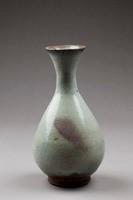
(a) Natural wheel-formed bowls
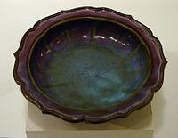
(b) Complex bowls with flower-like rims
Figure 1. Typical shapes of Jun ware
The typical shapes of Jun ware are presented in Figure 1. As shown in Figure 1(a), most Jun wares are natural wheel-formed bowls, small vases or wine-carafes, mostly with a narrow neck, but some are meipings (tall, with a narrow base, a wide body, a sharply-rounded shoulder, a short and narrow neck and a small opening) [2]. As shown in Figure 1(b), some Jun wares are made in double (two-part) moulds with more complex shapes. Many of the rims are irregular, forming flower-like shapes.
The shaping of Jun ware is a time-consuming procedure. On average, the ceramist needs to stay at the workbench for more than 8h a day. As a result, few people nowadays could like to inherit this traditional craftsmanship. To preserve such a valuable cultural heritage, it is imperative to develop a novel and effective digitalized shaping method for Jun ware.
Jun wares fall into two main groups: General Jun ware and Official Jun ware. The former refers to relatively popular wares with simple shapes, which were produced from Northern Song to Yuan dynasties. The latter, a much rarer type of Jun ware, was made for imperial palaces from Yuan to early Ming periods.
In view of the above, this paper designs a novel digital modelling strategy that captures and simulates the shape of Jun ware as a 3D computer model, which can be examined from multiple angles and edited easily with plug-in for 3D modelling software. The ordinary differential equation (ODE)-based modelling technique, which is known for its high accuracy, was introduced to simulate the complex curve surface and stitch up the connection parts produced by different moulds. The research findings shed new light on Jun ware design, facilitate 3D modelling of various Jun wares, and integrate computer graphics (CG) into digital production of the ware.
The remainder of the paper is organized as follows: Section 2 reviews the relevant studies on ODE-based swept surface modelling; Section 3 details the modelling of the two categories of Jun ware: The General Jun ware and the Official Jun ware; Section 4 applies the modelling strategy to specific examples; Section 5 wraps up this paper with meaningful conclusions.
The generation of swept surface has long been a hot topic in the field of CG. Bloor was the first to generate blend surface with partial differential equations (PDEs) [3]. John stone et al. [4] created a rational Bézier model of swept surface by interpolating key frames, without changing the curve shape at intermediate points. Focusing on the geometric modelling of human limbs, Hyun et al. [5] developed a modelling and deformation method based on swept surface and displacement map. Later, Hyun et al. [6] deformed polygonal grids of human models under the control of swept surfaces.
Swept surface generation is a parameterized modelling process [7-9], in which swept surfaces are constructed from a set of control parameters at a low computing cost. By the ODE method, a swept surface can be generated in four steps: formulating a vector-valued ODE, determining proper boundary conditions like boundary curves and boundary tangents, finding the solution to the vector-valued ODE, creating a profile curve (i.e. a generator), and sweeping the profile along the boundary curves while satisfying the boundary tangents at the same time by introducing the solution into the boundary conditions.
To satisfy the boundary conditions, both PDE and ODE approaches need to adopt a boundary value strategy, whereby 3D geometric models are reconstructed by analytical or numerical solution to PDEs/ODEs. The differential operators being selected form equations that may or may not obey certain physical laws. Such equations guarantee the orderly generation of surfaces from a known set of boundary conditions, which can be presented as a compact dataset. The property and shape of the generated surface can be altered by changing the equations and the boundary dataset.
For general PDEs, it is difficult to obtain analytical solutions. Thus, numerical solutions are sought instead, producing a numerical solver to customize surfaces. By contrast, the ODEs with constant coefficients can be solved analytically as far as the order is no greater than 6, making the computation highly efficient. Hence, the ODE offers an effective and powerful modelling method for our research.
In this paper, ODE-based swept surface is taken as the basis for the shape modelling of Jun ware. The geometric shapes of Jun ware were made editable based on Reference [10], where 3D models of Chinese marionette head are created through ODE-based geometric parameterisation and modelling.
The 3D model of Jun ware can be obtained by scanning. However, this method both consumes much labour and requires lengthy data processing (e.g. noise elimination and grid refinement). What is worse, the generated model cannot be reused unless the modeller has the special knowledge and skills on re-editing and reconstruction.
This section attempts to provide a user-friendly, efficient method to create various shapes of Jun ware with the aid of CG, enabling ordinary people to engage in this artistic creation. The Jun ware shape was simulated as parameterised swept surfaces, making the 3D model suitable for machining, the surface edition accurate and the connection between adjacent patches smooth.
3.1 Mathematical model
The ODE-based swept surface was adopted to simulate Jun ware shape, under the inspiration of Liang and You’s modelling of Chinese marionette head through ODE-based surface generation [10] and You et al.’s simulation of various objects by ODE-based swept surface method. In these studies, a 3D curve named generator is swept along two 3D trajectories, a.k.a. trim lines, to set up continuous blend surfaces with a controllable shape; the shape of the generator is controlled by a vector-valued 4th-order ODE. To keep the surfaces continuous, positional and tangential continuities are exactly satisfied at the trim lines. Below is a mathematical description of the above process.
A swept surface $\vec{F}=\vec{F}(u,v)$ is created to sweep across a profile curve $\vec{P}=\vec{P}(u,v)$ along two boundary curves ($\vec{B}_1$ and $\vec{B}_3$) under the constraints of boundary tangents ($\vec{B}_2$ and $\vec{B}_4$), which are defined at the boundary curves. The boundary curves and boundary tangents constitute four constraints that should be satisfied when the profile curve $\vec{P}$ sweeps to generate the swept surface F. The four constraints can be expressed as:
$\begin{align} & u=0:{{{\vec{B}}}_{1}}(v)=\vec{F}(0,v);{{{\vec{B}}}_{2}}(v)=\frac{\partial \vec{F}(0,v)}{\partial u}; \\ & u=1:{{{\vec{B}}}_{3}}(v)=\vec{F}(1,v);{{{\vec{B}}}_{4}}(v)=\frac{\partial \vec{F}(1,v)}{\partial u}; \\\end{align}$ (1)
where, $u$ and $v∈[0,1]$ are control parameters of the surface $\vec{F}$.
The 4th-order ODEs involve four unknown constants, namely, two boundary curves ($\vec{B}_1$ and $\vec{B}_3$) and the constraints of boundary tangents ($\vec{B}_2$ and $\vec{B}_4$). These constants can serve as the four constraints that must be satisfied when the profile curve sweeps to generate the swept surface.
To satisfy the four constraints, a 4-th order ODE was introduced for surface blending with positional and tangential continuities:
${{\vec{a}}_{1}}\frac{{{d}^{4}}\vec{P}(u)}{d{{u}^{4}}}+{{\vec{a}}_{2}}\frac{{{d}^{2}}\vec{P}(u)}{d{{u}^{2}}}=0$ (2)
where, $\vec{P}(u)$ is a vector-valued function of the generator; $a ⃗_1$ and $a ⃗_2$ are vector-valued material constants of the beam model. The material constants are called shape control parameters, and used as shape controllers for the generator.
Normally, the order of the ODE is positively correlated with the smoothness of the connection between two adjacent surface patches and the computing load. For instance, a 2nd order ODE guarantees zero-order continuity of the position constraints at the boundary, a 4th order ODE ensures 2nd order tangential continuity between adjacent surface patches, and a 6th order ODE maintains curvature continuity. Meanwhile, the computing load increases all the way from the 2nd order ODE to the 6th order ODE. Therefore, the 4th order ODE is selected for our research due to its good seam smoothness and moderate burden.
The vector-valued function of the generator (the profile curve) $\vec{P}(u)$ can be defined as:
$\bar{\vec{P}}(u)={{e}^{\vec{r}u}}$ (3)
For simplicity, formal operation notations were used to represent the operations of the components of vectors. For example, $a ⃗ $ is related to $a ⃗_1$ and $a ⃗_2$, $a=√|a_2/a_1|$ stand for $a_x=√|a_1x/a_2x|$, $a_y=√|a_1y/a_2y|$ and $a_z=√|a_1z/a_2z|$.
Taking each component of the vector-valued function of the generator $\vec{P}(u)$, the complementary solution of the vector-valued ODE Equation (2) can be rewritten as an algebraic equation
For $a ⃗_1$ and $a ⃗_2$ to have the same sign
$\bar{\vec{P}}(u)={{\vec{c}}_{1}}+{{\vec{c}}_{2}}u+{{\vec{c}}_{3}}\cos (\vec{a}u)+{{\vec{c}}_{4}}\sin (\vec{a}u)$
For $a ⃗_1$ and $a ⃗_2$ to have different signs
$\bar{\vec{P}}(u)={{\vec{c}}_{1}}+{{\vec{c}}_{2}}u+{{\vec{c}}_{3}}{{e}^{\vec{a}u}}+{{\vec{c}}_{4}}u{{e}^{\vec{a}u}}$ (4)
For$a ⃗_2$=0
$\bar{\vec{P}}(u)={{\vec{c}}_{1}}+{{\vec{c}}_{2}}u+{{\vec{c}}_{3}}{{u}^{2}}+{{\vec{c}}_{4}}{{u}^{3}}$
where $c ⃗_1$, $c ⃗_2$, $c ⃗_3$ and $c ⃗_4$ are unknown variables determined with boundary constraints. In fact, their values can be obtained by solving the constraints in Equation (1).
For example, substituting a solution to the profile curve $\bar{\vec{P}}(u)=c ⃗_1+c ⃗_2 u+c ⃗_3 cos( a ⃗u)+c ⃗_4 sin( a ⃗u) with a ⃗_1 a ⃗_2>0$ into Equation (2), the surface equation can be obtained as:
$\vec{F}(u,v)=\left( {{{\vec{c}}}_{1}}(v)+{{{\vec{c}}}_{2}}(v)u+{{{\vec{c}}}_{3}}(v)\cos (\vec{a}u)+{{{\vec{c}}}_{4}}(v)\sin (\vec{a}u) \right)$ (5)
If u=0 or u=1, the boundary constraints must be satisfied, yielding to the following expressions:
$\begin{align} & {{{\vec{c}}}_{1}}(v)={{{\vec{b}}}_{0}}\left( {{{\vec{b}}}_{1}}{{{\vec{B}}}_{1}}(v)+{{{\vec{b}}}_{2}}{{{\vec{B}}}_{2}}(v)+{{{\vec{b}}}_{3}}{{{\vec{B}}}_{3}}(v)-{{{\vec{b}}}_{4}}{{{\vec{B}}}_{4}}(v) \right) \\ & {{{\vec{c}}}_{2}}(v)={{{\vec{b}}}_{0}}\left( {{{\vec{b}}}_{5}}{{{\vec{B}}}_{1}}(v)+{{{\vec{b}}}_{3}}{{{\vec{B}}}_{2}}(v)-{{{\vec{b}}}_{5}}{{{\vec{B}}}_{3}}(v)+{{{\vec{b}}}_{3}}{{{\vec{B}}}_{4}}(v) \right) \\ & {{{\vec{c}}}_{3}}(v)={{{\vec{b}}}_{0}}\left( {{{\vec{b}}}_{3}}{{{\vec{B}}}_{1}}(v)-{{{\vec{b}}}_{2}}{{{\vec{B}}}_{2}}(v)-{{{\vec{b}}}_{3}}{{{\vec{B}}}_{3}}(v)+{{{\vec{b}}}_{4}}{{{\vec{B}}}_{4}}(v) \right) \\ & {{{\vec{c}}}_{4}}(v)=\frac{{{{\vec{b}}}_{0}}}{{\vec{a}}}\left( -{{{\vec{b}}}_{5}}{{{\vec{B}}}_{1}}(v)+{{{\vec{b}}}_{1}}{{{\vec{B}}}_{2}}(v)+{{{\vec{b}}}_{5}}{{{\vec{B}}}_{3}}(v)-{{{\vec{b}}}_{3}}{{{\vec{B}}}_{4}}(v) \right) \\\end{align}$ (6)
This means the sum of all profile curves forms the entire swept surface $\vec{F}(u,v)$:
$\begin{align} & \vec{F}(u,v)=\text{ }\!\!\{\!\!\text{ }\left( {{{\vec{b}}}_{1}}{{{\vec{B}}}_{1}}(v)+{{{\vec{b}}}_{2}}{{{\vec{B}}}_{2}}(v)+{{{\vec{b}}}_{3}}{{{\vec{B}}}_{3}}(v)-{{{\vec{b}}}_{4}}{{{\vec{B}}}_{4}}(v) \right) \\ & +\left( {{{\vec{b}}}_{5}}{{{\vec{B}}}_{1}}(v)+{{{\vec{b}}}_{3}}{{{\vec{B}}}_{2}}(v)-{{{\vec{b}}}_{5}}{{{\vec{B}}}_{3}}(v)+{{{\vec{b}}}_{3}}{{{\vec{B}}}_{4}}(v) \right)u \\ & +\left( {{{\vec{b}}}_{3}}{{{\vec{B}}}_{1}}(v)-{{{\vec{b}}}_{2}}{{{\vec{B}}}_{2}}(v)-{{{\vec{b}}}_{3}}{{{\vec{B}}}_{3}}(v)+{{{\vec{b}}}_{4}}{{{\vec{B}}}_{4}}(v) \right)\cos (\vec{a}u) \\ & +\left( -{{{\vec{b}}}_{5}}{{{\vec{B}}}_{1}}(v)+{{{\vec{b}}}_{1}}{{{\vec{B}}}_{2}}(v)+{{{\vec{b}}}_{5}}{{{\vec{B}}}_{3}}(v)-{{{\vec{b}}}_{3}}{{{\vec{B}}}_{4}}(v) \right)\sin (\vec{a}u)\}/{{{\vec{b}}}_{0}} \\\end{align}$(7)
where,
$\begin{align} & {{{\vec{b}}}_{0}}=2-2\cos \vec{a}-a\sin \vec{a} \\ & {{{\vec{b}}}_{1}}=1-\cos \vec{a}-\vec{a}\sin \vec{a} \\ & {{{\vec{b}}}_{2}}=\cos \vec{a}-\vec{a}\sin \vec{a} \\ & {{{\vec{b}}}_{3}}=1-\cos \vec{a} \\ & {{{\vec{b}}}_{4}}=1-\vec{a}\sin \vec{a} \\ & {{{\vec{b}}}_{5}}=\vec{a}\sin \vec{a} \\\end{align}$.
Equation (7) lays the basis for swept surface generation. Using 3D modelling software like Autodesk Maya, the boundary points can be selected manually for information extraction from boundary curves [11, 12].
3.2 Shape modelling of general Jun ware
General Jun wares are mostly simple in shape and decorations, which are limited to the glaze effect. The walls are thick and sturdy. Most General Jun wares are natural wheel-formed bowls and dishes, and small vases or wine-carafes, mostly with a narrow neck. There are also boxes, jars, ewers and other shapes.
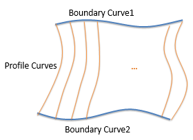
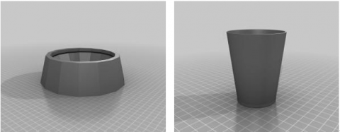
Considering the simple shape, the ODE-based swept surface was employed to model General Jun ware. First, a swept surface was created with two open boundary curves (Boundary Curves 1 and 2 in Figure 2(a), where the profile curves $\bar{\vec{P}}(u)$ at v=0 and v=1, form two open edges. Sweeping a profile curve along the two boundaries, a set of profile curves were generated as bone structures for the swept surface. As shown in Figure 2(b), the 3D shapes of two General Jun wares were created by sweeping profile curves (the generators) along open boundary curves under boundary tangents.
(a)
(b)
Figure 2. Swept surfaces generated by open boundary curves
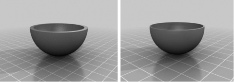
A degeneration surface of open boundary curves is shown in Figure 3(a), where one boundary curve (Boundary Curve 1) shrinks into a single point and the parameter increases from 0 to 1. As shown in Figure 3(b), the 3D shapes of two General Jun wares were generated by sweeping a profile curve (the generator) along one boundary curve and one degeneration boundary curve under the boundary tangents. The boundary curve and the degeneration boundary curve had the same point coordinates.
(a)
(b)
Figure 3. Swept surfaces generated by open boundary curve and a single point
3.3 Shape modelling of official Jun ware
Compared with the General Jun ware, Official Jun ware are larger, heavier with more complex shapes. Many Official Jun wares have irregular, flower-like rims and incisions on the bases. Obviously, the complex details of Official Jun ware require more complicated swept surfaces to simulate than the simple shape of General Jun ware.
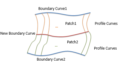
In fact, the primary shape of a Jun ware can be edited either by changing the boundary conditions or by altering profile curves controlled by parameter $a ⃗_1$ and $a ⃗_2$ in Equation (2) [13]. The existing surface should be divided into smaller pieces to refine the local features of the swept surface and create the effect of irregular rims. For example, the surface Figure 2(a) can be split into two patches in the following means.
For a known surface with boundary conditions, all the points on the profile curves have same u value, which form a new curve (the red curve in the middle of Figure 4(a)). This new boundary curve, coupled with the known boundary conditions, two surfaces (Patch 1 and Patch 2 in Figure 4 (a)) can be generated, with the same shape as the old surface. Each of the two new surfaces can be further refined by adjusting the boundary conditions.
The 3D shapes of two Official Jun wares were obtained by refining the existing surface generated for one General Jun ware. Through local refinement of the swept surface, the flower-like rims were simulated as Figure 4(b).
(a)
(b)
Figure 4. An example of shape modelling of Official Jun ware
The common way to model the shape of Jun ware is to convert a scanned mesh of an existing Jun ware into ODE surfaces. Firstly, a real Jun ware should be scanned into polygon grids. Then, the grids should be imported into the computer to obtain ODE patches. The scanned model often has unstructured data, which are not suitable for 3D modelling without laborious noise removal and grid refinement.
In this paper, a 3D shape modelling method is proposed for Jun ware. Through the following steps, our method enables common people to produce Jun ware referring to images or initial design.
Step 1. Approximate the desired shape by sweeping a profile curve (the generator) along two boundaries curves by the ODE method;
Step 2. Alter the boundary curves by adjusting the shape control parameters $a ⃗_1$ and $a ⃗_2$, two shape controllers for the generator, with special attention paid to areas related to the adjacent patches;
Step 3. Refine the shape surface locally by inserting new boundary curves, in an attempt to simulate the complex features of Official Jun ware;
Step 4. Adjust the boundary curves related to the newly inserted patches in Step 2;
Step 5. Remove the undesirable patches;
Step 6. Go back to Step 2 and refine the model, or go back to Step 1 and modify the outline of the model if the shape is not satisfactory.
Step 7. Finalise the Jun ware model.
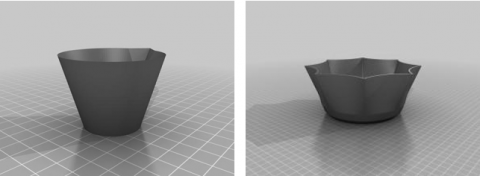
Through the above steps, the author created surface models for both General Jun ware and the Official Jun ware with complex shapes. Generally, a manually generated Jun ware model needs thousands grids to approximate the shape. After all, a model with fewer grids may have poor quality and retain few surface details. In our method, the shape can be controlled with a few parameters. For example, a handful vertices is needed to store the boundary conditions for shaping (Figure 5).
Figure 5. Jun ware models with complex shapes
Considering the immense value and preservation difficulty of Jun ware, this paper designs a novel digital modelling strategy that captures and simulates the shape of Jun ware as a 3D computer model, which can be examined from multiple angles and edited easily with plug-in for 3D modelling software. The ODE-based modelling technique, which is known for its high accuracy, was introduced to simulate the complex curve surface and stitch up the connection parts produced by different moulds.
Our method enjoys the following advantages: the swept surface can provide a lightweight analytical model to simulate the Jun ware shape, making the representation efficient and numerically robust; the surface model can be easily modified and regenerated by editing the profile curves and boundary curves, reflecting the various shapes of both General and Official Jun wares; the parameterised swept surface generation model requires a few vertices to store the boundary conditions for shaping. Our novel modelling approach keeps Jun ware design simple and engaging to young craftsmen.
The future research will improve the proposed method with more sophisticated techniques and CG tools. The goal is to further simplify the design and preserve the value of Jun ware.
The research leading to these results has received funding from the National Natural Science Foundation of China (NSFC, 61872439). The authors acknowledge partial support from Henan Joint International Research Laboratory of Design Presents Virtual Simulation and the Key Scientific Research Projects of Henan Province of China (182102210155).
[1] Vainker SJ. (1991). Chinese pottery and porcelain. British Museum Press, 9780714114705.
[2] Bloor M, Wilson M. (1989). Generating blend surfaces using partial differential equations. Computer-Aided Design 21(3): 165-171. http://dx.doi.org/10.1016/0010-4485(89)90071-7
[3] Johnstone JK, Williams JP. (1995). A rational model of the surface swept by a curve. Computer Graphics Forum 14(3): 77-88. http://dx.doi.org/10.1111/1467-8659.1430077
[4] Hyun DE, Yoon SH, Kim MS, Juttler B. (2003). Modeling and deformation of arms and legs based on ellipsoidal sweeping. 11th Pacific Conference onComputer Graphics and Applications, 2003. Proceedings, pp. 204-212. http://dx.doi.org/10.1109/PCCGA.2003.1238262
[5] Hyun DE, Yoon SH, Chang JM, Seong JK, Kim MS, Juttler B. (2005). Sweep-based human deformation. The Visual Computer 21(8-10): 542-550. https://doi.org/10.1007/s00371-005-0343-x
[6] Parke F. (1972). Computer generated animation of faces. In Proceedings of the ACM Annual Conference 1: 451-457. https://doi.org/10.1145/800193.569955
[7] Ehsani H, Poursina, M, Rostami M, Mousavi A, Parnianpour M, Khalaf K. (2019). Efficient embedding of empirically-derived constraints in the ODE formulation of multibody systems: Application to the human body musculoskeletal system. Mechanism and Machine Theory 133: 673-690. https://doi.org/10.1016/j.mechmachtheory.2018.11.016
[8] Asai Y, Kloeden PE. (2019). Numerical schemes for ordinary delay differential equations with random noise. Applied Mathematics and Computation 347: 306-318. http://dx.doi.org/10.1016/j.amc.2018.11.033
[9] Liang H, Chang J, Yang X, You L, Bian S, Zhang JJ. (2015). Advanced ODE based head modelling for Chinese marionette art preservation. Computer Animation and Virtual Worlds 26(3-4): 207-216.
[10] You L, Ugail H, Tang B, Jin X, You X, Zhang JJ. (2014). Blending using ODE swept surfaces with shape control and C^1 continuity. The Visual Computer 30(6-8): 625-636. https://doi.org/10.1007/s00371-014-0950-5
[11] You L, Yang X, Pachulski M, Zhang JJ. (2007). Boundary constrained swept surfaces for modelling and animation. Computer Graphics Forum. Blackwell Publishing Ltd 26(3): 313-322. http://dx.doi.org/10.1111/j.1467-8659.2007.01053.x
[12] You L, Yang X, You X, Jin X, Zhang JJ. (2010). Shape manipulation using physically based wire deformations. Computer Animation and Virtual Worlds 21(3-4): 297-309. http://dx.doi.org/10.1002/cav.352
[13] Christie's NY. (2016). The classic age of Chinese ceramics: The Lin Yu Shan Ren Collection, Part II. New York, Rockefeller Plaza.