Guglielmina Mutani* | Silvia Santantonio | Angelo Tartaglia
OPEN ACCESS
The objectives of the European Energy transition entail an increasing use of electricity especially for residential sector. Member states are invited to promote energy policies that involve stakeholders directly. Energy Communities (EC) are intended as local institutions that could drive this change, creating local-scaled energy entities that cooperate to exchange energy. The purpose of this study is to investigate the energy consumption identifying a linear regression model to forecast electric energy demand at municipal scale, for residential end users. This work analyses electric consumption of 1,201 municipalities in Piedmont (north-west of Italy) evaluating the main energy-related variables. Information are obtained by online databases and georeferenced with GIS tool. The identified model evidences that the most influential variables are the population, the number of members per family, the education level, and the income. Regarding building features, the dwelling area and the number of occupied dwellings, the age of buildings and their maintenance condition. The statistical GIS-based methodology proposed in this study is replicable and can be applied to other contexts. A forecasting model to predict the amount of energy demand can support preliminary decision-making process defining the scale of ECs and their optimal configuration for balancing energy demand and local production.
electric consumption, residential user, linear regression, statistical model, place-based assessment, municipal data, territorial scale
Since recent years, global climate change has raised concerns about the sustainability of energy supply systems and the depletion of resources. The decarbonization objectives [1] envisage an increasing use of electric energy in all sectors. Especially for residential users, the dependence on electricity has been increasing, partly because of the computerization of every-day life, partly due to the conversion to this energy vector for uses not previously contemplated.
The residential end-use sector on energy consumption impacts largely on the total national electric consumption, reaching top percentages in most developed countries [2]. However, compared to other end-use sectors, as industrial, commercial and transportation, the residential one has been described as “largely undefined energy sink” [3]. Swan and Ugursal [3] explained that not only building characteristics, but also occupant behaviour data are needed to understand deeper residential consumption, but privacy issues in collecting data and the prohibitive cost of such surveys contribute to the poor understanding of this part of electric consumption.
The fulfilment of the European energy transition goals of energy savings and security is a current issue in the agenda of governments. Local energy policies must consider economics and environmental concerns and it is essential to better understand residential energy demand characteristics to define proper solutions for each territory.
So far, the main strategies envisaged are based on the provision of economic incentives to single user for energy efficiency measures and for the installation of renewable energy sources (RES) production plants. To foster the achievement of these objectives and to make citizens active part of change in new ways, strategies have been recently implemented and new aggregation models of energy users have been defined.
European Community looks at the municipality as the local institutions which could drive this change, with the creation of new local-scaled energy entities, as the definition of Energy Community (EC) suggests [4].
As defined by [4] a local EC is a non-profit organization of final customers, which can involve different local stakeholders (municipalities, citizens, public and private companies) with the aim of achieving energy independence and security, a sustainable development and affordable energy costs. These objectives can be reached through energy efficiency interventions, exploitation of local RES, implementation of local energy grids to obtain smarter, flexible, and resilient configurations. The recognition of the prosumer is of fundamental importance for the optimal configuration of the EC. The balanced composition of stakeholders, in terms of energy demand amount and production profiles, can ensure the optimization of energy exchange between members, with economic and environmental advantages for all.
The Clean Energy Package contains two energy community (EC) definitions: Citizen Energy Community (CEC), in Electricity Directive 2019/944, and Renewable Energy Community (REC), in Renewable Directive 2018/2001. Both directives describe EC as a collective cooperation of energy related activities around specific ownership, governance, and non-commercial purpose. RECs may be considered a subset of CECs that promote the use of renewable energy sources. Member States facilitate energy communities in accessing to incentives and information, assisting vulnerable and low-income households, and removing, when possible, regulatory and administrative barriers.
Regardless of the various legal and economic models, ECs can be intended as regional developments that involve citizens, social entrepreneurs, public authorities, and community organizations in producing, selling, and distributing renewable energy [5]. As promising social instruments, Ecs can participate directly in the energy transition, offering a bottom-up path to energy efficiency and low-carbon systems [6].
To realize EC, considerations in urban planning have to be made, and energy consumption has to be investigated at a local scale [7].
This work aims to evaluate the electric energy consumption of residential end users at local level, using the main energy-related variables. The purpose is to define a replicable methodology based on multiple linear regression model able to predict residential annual electric consumption at municipal scale.
The analysis has been performed using a Geographical Information System (GIS) tool and a statistical software. The GIS tool has been used for the association of different databases, and for calculating climatic and environmental variables. The statistical software allowed to implement statistical techniques as principal components analysis and multiple linear regression to evaluate the main energy-related variables and the electric consumption models for municipalities.
Reducing and rationalizing electric consumption for residential use is an important issue in the agenda of governments and decisions makers, and studies have tried to understand the main environmental and socio-demographic variables that influence electric energy consumptions at different scales.
In 2009, Olofsson et al. [8] analysed the effect of building-specific features on both thermal and electric energy consumption using analysis of variance (ANOVA) tests. They stated that the most important variables were the geometrical characteristics and the construction time of the buildings. However, Howard et al. [9] in 2012 applied a multiple linear regression model that evidenced the higher importance of building function than the construction type or age of construction.
Two studies conducted in Rotterdam (Netherlands) [10, 11] in recent years, using a multiple linear regression model to investigate both natural gas and electric consumption, pointed out that for electricity number of occupants, floor surface and type of dwelling are the most significant variables. Furthermore, Nouvel et al. [11] compared an engineering method to a statistical one to predict electric consumption from average floor area of dwellings, average number of occupants and the share of dwellings. They showed that the deviation from real energy consumption data was lower using a statistical approach.
In 2019, Mutani et al. [12] evaluated the thermal consumption of building in the urban context of Torino (Italy). They implemented a multiple linear regression model, using building-specific features as well as environmental and socio-demographic variables, that allowed to highlight major drivers of the energy consumption as area of dwellings, number of occupants, but also age of the residents and their social characteristics.
Chen et al. [13], used a multiple regression analysis to investigate the relationship among household variables and residential energy consumption for space heating and cooling. Data were obtained from more than 1,500 surveys applied to households in the city of Hangzhou (China). The results pointed out that up to 28.8% of the energy consumption could be explained by socio-economic and behavioural variables, and floor area accounts for 44%.
Bianco et al. [14] analysed residential and non-residential annual electric consumption in Italy, during the period 1970–2007. They implemented simple and multiple regression models using historical data on energy consumption, gross domestic product (GDP) and GDP per capita and demographic data.
In 2013, Gans et al. [15] used data on real-time usage from Continuous Household Survey of Northern Ireland, which surveyed about 300 households per month, to investigate the effect on residential electric consumption. The surveys collected socio-economic data as dwelling, health, education, employment, and welfare payments. The regression model implemented accounted electricity price, household income as well as weather, house-specific features, and type of heating system.
Nie and Kemp [16] investigated trends in energy consumption in China during the 2002-2010 years, obtaining data from open-access institutional databases. They evaluated the effect of changes in demographic parameters, house-specific characteristics, technology systems and energy sources. The key drivers for energy consumption increase were appliances, floor space per capita, whereas the energy mix and population were the less significant. They tried to forecast electric use using the regression method, predicting that the electric consumption would continue to rise despite a partial saturation of the demand.
Social, demographic, and economic variables, along with environmental and building-specific features are useful to understand electric consumption for the residential sector and even to forecast future trends. On the other hand, in-field collection of data from surveys and measurement are costly and time-consuming and cannot be performed on a vast scale. Therefore, the aim of this study is to identify the most influential variables on electric energy consumption for residential sector at a municipal scale, starting from public-access data.
The case study analysed in this work consist in the data sample of the 1,206 municipalities in Piedmont Region, in the North-West of Italy. The territory is considered according to its climatic-environmental, socio-economic characteristics, and those related to the built environment. This information was georeferenced using the GIS tool and was obtained from the online database Geoportale Piemonte (technical regional map BDTRE, updated to 2019) [17], the Digital Terrain and Surface Models (DTM and DSM), and the Italian census database (ISTAT 2011) [18]. For all characteristics individuated, in Table 1 are shown the main statistical parameters evaluated for each municipality analysed. In the pre-processing phase, the presence of incomplete information and outliers has been checked, and the municipalities of which has been removed (5 outliers: the city of Turin, the municipalities of Novara and Alessandria; 2 municipalities with incomplete data: Vercelli and Valpratosoana). The vast area of the region (25,387 km2) with its heterogeneous morphology, includes different types of environmental context: mountains, hills, and plain areas and an altitude that has an average value of 421 m asl. From the climatic data provided by the Regional environmental protection agency (ARPA), the Heating Degree Days (HDD) were obtained from the UNI 10349-3:2016, and the corresponding climatic zone has been assigned to each municipality (E 1-3 and F 1-4, see Table 2), according to previous work [19]. There are 892 municipalities in the climatic zone E (i.e. HDDE < 3000 °C) and 309 in zone F (i.e. HDDF ≥ 3000 C), that respectively represent the 74% and the 26% of all municipalities. The total population in Piedmont is 4,363,916 inhabitants (ISTAT 2011), with an average population density equals to 153 inh/km2. Seven categories of population (P) were defined to create homogeneous groups between municipalities (LP-Low, MP-Medium, HP-High). Table 2 shows the number of municipalities belonging to population and climatic zones categories.
Table 1. Geo-climatic-environmental, socio-economic, built heritage characteristics of the case study
|
Characteristics |
Statistical parameters |
||||
|
Climatic-environmental |
min |
max |
median |
average |
|
|
Area [km2] |
0.7 |
203.7 |
13.4 |
21.0 |
|
|
Altitude [m asl] |
76.0 |
2,035.0 |
334.0 |
420.4 |
|
|
HDD [°C/yr] |
2,422 |
5,165 |
2,766 |
2,883 |
|
|
Socio-economical |
|
|
|
|
|
|
Population [no. inhab] |
42 |
101,952 |
1,015 |
2,868 |
|
|
Density [inhab/ km2] |
0.5 |
2,830.8 |
81.4 |
153.0 |
|
|
Foreigner [% on tot pop] |
0 |
22.3 |
5.4 |
6.1 |
|
|
Age [% on tot pop] |
0-19 /20-69 /70-99 |
16 /64 /20 |
16 /64 /20 |
16 /65 /19 |
16 /64 /20 |
|
Education Diploma [% on tot pop] |
Primary School /Jr. High School /Sr. High School /University |
8 /18 /10 / 0 |
57 /49 /50 /30 |
27 /35 /30 / 7 |
28 /34 /30 / 8 |
|
Occupation
|
Workforce (W) /NoW [% on tot pop] |
22 /33 |
66 /77 |
51 /49 |
51 /49 |
|
|
Employed (E) /NoE [% on tot W] |
8 / 0 |
100 / 20 |
95 / 5 |
95 / 5 |
|
|
Homemakers /Students / Fixed income /Others [% on tot NoW] |
2 / 0 /24 / 0 |
38 /26 /88 /31 |
16 /11 /65 / 8 |
15 /11 /66 / 8 |
|
Income |
[€/yr/n. of taxpayer] |
6,737 |
36,415 |
19,436 |
19,367 |
|
Families [% on tot n.] |
1 member / 2 members / 3 members / 4 members / 5 members / 6 or more members |
16 /12 / 1 / 0 / 0 / 0 |
81 /41 / 32 / 24 / 10 / 4.8 |
35 /29 /19 /12 / 2.6 / 0.7 |
38 /28 /18 /12 / 2.6 / 0.8 |
|
Residential Built Heritage |
|
|
|
|
|
|
Year of construction [% on tot buildings] |
Before 1918 1919 – 1945 1946 – 1960 1961 – 1970 1971 – 1980 1981 – 1990 1991 – 2000 2001 – 2005 After 2005 |
0 / 0 / 0 / 0 / 0 / 0 / 0 / 0 / 0 |
98 /91 /63 /44 /59 /46 /25 /18 /21 |
34 /12 / 8 /10 /10 / 5 / 4 / 2 / 2 |
37 /16 /10 /11 /11 / 6 / 4 / 3 / 2 |
|
Number of floors [% on tot buildings] |
1 floor / 2 floors / 3 floors / 4 or more floors |
0 / 1 / 0 / 0 |
97 /96 /82 /72 |
7 / 62 /24 / 2 |
9 /61 /25 / 4 |
|
Maintenance condition [% on tot buildings] |
Optimal / Good / Mediocre / Worst |
0 / 1 / 0 / 0 |
98 /99 /80 /23 |
29 /50 /14 / 1 |
31 /51 /16 / 2 |
Table 2. Municipalities in P and climatic zone categories
|
Climatic Zone |
LP |
MP |
HP |
||||
|
p<350 |
350<p<750 |
750<p<1500 |
1500<p<3000 |
3000<p<5000 |
5000<p<50000 |
p>50,000 |
|
|
E1 |
2 |
3 |
14 |
8 |
4 |
5 |
1 |
|
E2 |
32 |
68 |
92 |
86 |
38 |
65 |
3 |
|
E3 |
65 |
110 |
125 |
80 |
47 |
44 |
- |
|
F1 |
77 |
49 |
33 |
25 |
16 |
12 |
1 |
|
F2 |
37 |
18 |
11 |
1 |
1 |
- |
- |
|
F3 |
12 |
4 |
1 |
- |
1 |
- |
- |
|
F4 |
7 |
1 |
2 |
- |
- |
- |
- |
The average age of the population is 48 years and foreigners represent on average the 6.1% of the total municipal population. On average, there are 2.15 persons per family. Residential buildings in each municipality represent 91% of the total number of buildings and 66% of them is occupied, with an average total floor area of 106.63 m2 and an average floor area for each person equal to 49.6 m2.
In this work, the energy data refer to the annual electricity consumption of the residential sector of the 1,206 Piedmont municipalities. Considering the ones with complete information, 1,201 municipalities were selected with annual energy consumption data, from 2010 to 2016.
To investigate major drivers of residential electric consumption, a GIS-based methodology with the implementation of statistical techniques has been developed in this study. The achievement of the best accuracy depends on the reliability of data and databases. In this study, to enhance pragmatism and ensure reproducibility, variables were obtained from institutional open-access databases [17-19], geographical and environmental data were calculated using well established procedure with GIS software [20, 21], while electric consumption observations were obtained from the database provided by the Piedmont Region technical office, which collects energy data directly from the Distribution System Operators (DSOs) [22].
The software used was R version 4.0.0 with a database composed by 1,201 observations and 117 variables related to residential electric consumptions. The observations consist in the yearly consumption of 1,201 municipalities from 2010 to 2016 (6 years), excluding the year 2011 because of missing data. Variables were collected only once for each municipality, assuming that during the time span considered they did not vary significantly. The methodological framework of this study can be summarized in the following steps:
4.1 Statistical distribution of energy consumption data
Considering 1,201 municipalities, statistical analysis was performed to evaluate the frequency distribution of energy consumption data separately for each of the six-year span. Anomalous observations were individually evaluated, comparing the consumption of each year to the previous and the next ones. Cut-off for maximum variation was set arbitrarily to 0.3. Observation that varied more than 30% were eliminated. The final database consists of 1,186 municipalities selected. Cullen and Frey chart has been used to inspect plausible probability distribution.
The Normal and Log-Normal distributions were checked by graphically evaluating the goodness of fit, drawing probability density functions and histogram together [23]. The ANOVA test has been used for evaluating whether the electric consumption differs significantly among years.
4.2 Identification of independent variables
Residential electric energy consumption of 1,186 municipalities were georeferenced using a GIS tool, to combine the energy consumption data with the socio-demographic and environmental characteristics of the municipalities. The socio-economic and built environment characteristics refer spatially to the census sections, which represent the territorial units commonly used to collect data. In this work, the 2011 ISTAT census database has been managed using GIS tool referring all available information to the municipal area. Some variables have been transformed: the values of some observations (absolute values) have been calculated in percent of the total value, new variables were created from the former variables.
4.3 Univariate and multivariate analysis techniques
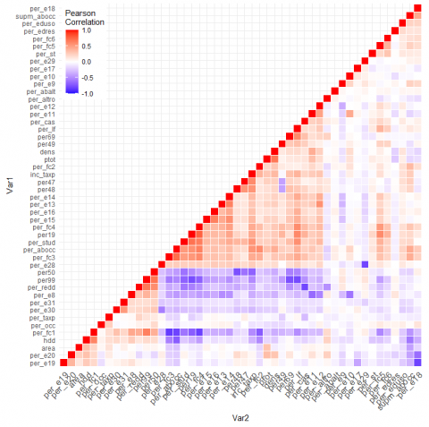
First, univariate statistical methods were used to describe and investigate variables and their relationship with the outcome. Pearson’s rho [r] was used to assess the level of correlation among variables and between each variable and the electric consumption data. A correlation matrix was used to identify collinear variables and remove them from subsequent analysis to avoid singularity of the correlation matrix itself.
The principal component analysis (PCA) was used to identify variables that are able to explain the majority of data variability and to divide observations into homogeneous groups. The Kaiser-Meyer-Olkin factor has been referred as a measure of adequacy of PCA. Hierarchical clustering has been performed using on the selected principal components the criterion of Ward that is based on the multidimensional variance. To obtain homogeneous groups the cluster dendrogram, obtained from the PCA, has been cut off at the height of 1.0. The contribution of variables to main principal components was graphically evaluated to identify uninfluential variables.
Multiple linear regression models
The linear regression model is the most used statistical technique for investigating and modelling the relationship between a dependent and two or more independent variables. The electric energy consumption was estimated using a linear regression, which is expressed by Eq. (1):
$Y_{i}=\beta_{0}+\beta_{1} \cdot x_{i 1}+\cdots+\beta_{p} \cdot x_{i p}+\varepsilon_{i}$ (1)
where, Yi is the annual electric consumption (dependent variable), xij are the independent variables, $\beta_{\mathrm{i}}$ are the estimated coefficients and εi correspond to the random errors of each observation i, i=1, …, N. The standard errors must be independent and normally distributed with mean 0 and constant variance: εi ~IIND (0, σ2).
The Ordinary Least Squares (OLS) method was used to identify the model express by Eq. (1). The observed values yi (i=1, …, N) can be written as Eq. (2):
$y_{i}=b_{0}+b_{1} \cdot x_{i 1}+\cdots+b_{\mathrm{p}} \cdot X_{\mathrm{ip}}+e_{i}$ (2)
where, bj are the least squares estimates of βj (j=0,1, …, p) and ei (i=1, …, N) are the residuals. Predicted values yi are computed as b0 + b1 ∙ xi1 + ⋯ + bp ∙ xip (i=1, …, N).
Linear dependency, no multicollinearity among variables, normality of εi, and homoscedasticity among εi are the conditions on a multiple linear regression model.
The stepwise method in both directions (backward and forward) was performed to identify the linear model minimizing the Akaike information criterion (AIC), that is asymptotically equivalent to cross validation, and selecting the most influential variables. The stepwise method is an automatic selection procedure which combines backward elimination steps (computing the t-ratio for each regressor in a subset and eliminating the ones that have absolute value of the t-ratios smaller than a prespecified value) and forward selection steps (adding a new variable if the corresponding t-ratio is the largest and its value is greater than a prespecified value).
The models resulted from the stepwise must be checked, evaluating the residuals for their normality and homoscedasticity, and the variables for multicollinearity by their Variance Inflation Factor (VIF).
Homoskedasticity (homogeneous variance for residuals) is a crucial assumption in regression analysis. It was tested through the scatter plot of residuals predicted values, normality, and probability graphs (Q-Q-plot). The outlier and leverage diagnostic graphs have been used to identify observations that are influential points. Observations, whose residuals (Student residuals) and leverage values were higher than 2 standard deviations, have been selected and removed from the dataset and the analysis was performed again.
The appropriate diagnostics (e.g., Breusch–Pagan test and White test) were performed to check the accuracy of the model prediction. To evaluating homoscedasticity of residuals the White test has been conducted, considering the following hypotheses:
$H_{0}: \sigma_{i}^{2}=\sigma^{2}$ (3)
$H_{1}: \exists_{i, j}$ such that $\sigma_{i}^{2} \neq \sigma_{j}^{2}$ (4)
where, the null hypothesis (Eq. 3) implies that residuals have constant variance (σ2) and it is similar across all the values without showing any pattern, while the alternative hypothesis (Eq. 4) signifies a different variance among them. In this latter case a variance-stabilizing transformation is required to obtain more accurate variables estimators of the model.
The presence of heteroscedasticity in the final model was reduced through Heteroskedasticity-Consistent Standard Errors (HCSE or White correction), that allowed the fitting of a linear regression model that contains heteroscedastic residuals [24].
The multicollinearity of a multiple regression model makes difficult to understand how much the dependent variable is affected by the independent variables since they are all influencing each other. The validity of the multiple regression was assessed by the Variance Inflation Factors (VIF). It is calculated as the reciprocal of the inverse of Rj2 (where R2 is the coefficient of determination) of an independent variable xj as it is expressed by Eq. (5):
$V I F_{j}=\frac{1}{1-R_{j}^{2}}$ (5)
The VIF gives the proportional increase in the variance of $\beta_{i}$ with respect to what it would have been if the explanatory variables were completely uncorrelated. The evaluation criterion refers to the threshold calculated as Eq. (6)
$V I F<\max \left(10, \frac{1}{1-R_{\text {model }}^{2}}\right)$ (6)
where, $R_{\text {model}}^{2}$ is the usual R-squared of the regression model. Variables with high VIF have been transformed or redefined and analysis was performed again.
The coefficient of determination R2 correspond to the proportion of the variance in the dependent variable that is predictable from the independent variables and it was used to evaluate the adequacy of the model. The adjusted R2 (Adj R2) has been adjusted for the number of predictors in the model. R2 increases with the addition of variables in the model, while Adj R2 increases only if that addition improves the model more than would be expected by chance.
In this study, the transformation of variables in order to improve the accuracy of the model consisted in three types of intervention.
$z_{i j}=\frac{x_{i j}-\bar{x}_{j}}{\sigma_{j}}$ (7)
where, $\bar{x}_{j}$ is the mean of the jth variable and σj its standard deviation {xij: i=1, …, N};
Particularly, this latter is the case for the variables related to three characteristics of the population (Education degree, Family members and Age) and one characteristic of residential building (Building Construction Year).
Education degree variables. The 4 initial variables selected for the linear model consisted of the percentage of the population with different education levels: primary school diploma (P), junior high school diploma (JH), senior high school diploma (SH) or university degree (U); these variables were calculated as % values relative to the total population Ptot of each municipality. Each of them has been associated with the total number of years of study envisaged by the Italian school system, respectively: 5, 8, 13 and 18 years. Then the 4 variables have been redefined in a single variable (EDU) that expresses the average number of years of education of the population of the municipality, calculating the weighted average as Eq. (8):
$E D U=\frac{\operatorname{Ptot} *[(P * 5)+(J H * 8)+(S H * 13)+(U * 18)]}{P t o t}$ (8)
Family members variables. The 5 initial variables selected consisted of the percentage of the families with 1, 2, 3, 4, or 5 members per family relative to the total number of families (Ftot) of each municipality. Then the 4 variables have been redefined in a single variable (FAM) that expresses the average number of members per family for each municipality, calculating the weighted average.
Age variables. The 3 initial variables selected for the initial model consisted of the percentage on the total population (Ptot) that had 0-19, 20-69 or 70-99 years old. Then the 4 variables have been redefined in a single variable (AGE) that expresses the average age of the population in each municipality, considering the median value for each of the 3 starting age categories and calculating the weighted average.
Building Construction Year variables. The 9 initial variables selected for the initial model consisted of the percentage on the total number of residential building in each municipality that have been built respectively before 1918, 1919-1945, 1946-1960, 1961-1970, 1971-1980, 1981-1990, 1991-2000, 2001-2005, after 2005. Then the 9 variables have been redefined in a single variable (BCY) that expresses the average age of residential buildings in each municipality. The oldness of building has been identified as the difference between the corresponding year of energy data (2015) and the median value for each of the 9 starting categories, then the weighted average has been calculated.
4.4 Influence of independent variables
A further verification of the validity of the model took place by checking whether the observed values fall within the interval of the predicted values. Firstly, the predicted values for the year 2015 and the respective 95% confidence interval were calculated. The prediction interval was then calculated. This information was graphically evaluated in comparison with the observed values of the annual electricity consumption for the year 2010, 2012, 2013,2014,2016. For each of the 5 years, the observations that fell outside the prediction interval were identified. The information relating to them (e.g., belonging to the clusters and other variables) was obtained and their distribution was assessed.
In this paragraph the results are presented according to the steps of the methodological framework previously described.
5.1 Statistical distribution of energy consumption data
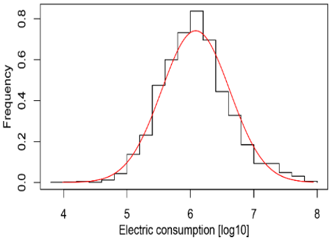
The statistical distribution of raw energy consumption data was not normal. Therefore, electric consumption has been log-transformed. Logarithmic distribution was evaluated approximately normal by the goodness of fit graph (Figure 1a), comparing the histogram of the outcome distribution with the probability density function (red line) of a normal distribution.
(a)
(b)
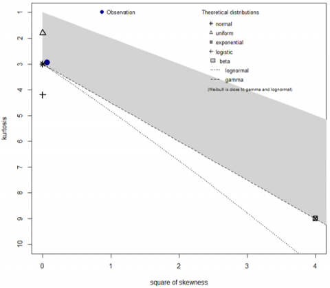
Figure 1. Goodness of fit graph(a) and Cullen-Frey chart(b).
The Cullen and Frey chart (Figure 1b) confirms the Log-normal distribution of the outcome (blue point) as it is compared to several theoretical distributions (asterisk). The log of the annual electric consumption is not significantly different among the six years (p-value: 0.271). Distribution of each year has been evaluated, Figures 1 (a, b) show the results of 2015.
5.2 Identification of independent variables
The variables identified and used to describe the electric consumption of residential users at municipal scale were 117 (114 numerical and 3 categorical) and they were synthesized in Table 3: for each characteristic is indicated the number of variables evaluated in the subsequent analysis; the asterisk indicates variables for which percentage has been calculated.
5.3 Univariate and multivariate analysis techniques
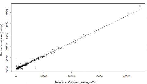
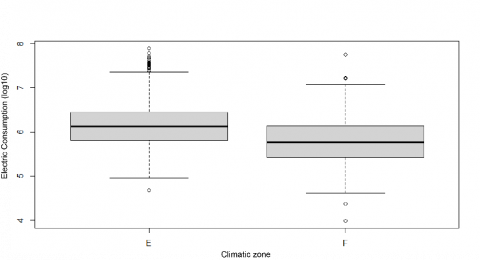
The trend of the socio-economic variables corresponds to a linear association to the electric consumption, and the same happens evaluating the number of occupied dwellings (Od) (Figure 2a). The electric consumption of municipalities in climatic zone E and F is significantly different (p-value< 0.0001), according to results of the Wilcoxon rank sum test with continuity correction. The difference of the energy consumption among municipalities in the same climatic zone is less than the one between the two zones. It means that the belonging to climatic zone affects significantly and not accidentally the energy consumption. In Figure 2b is evident that municipalities in zone F have a higher electric consumption than the ones in zone E.
Table 3. Characteristic considered in the database and number of variables selected for each feature
|
Climatic-Environmental |
Socio- economic |
Residential built heritage |
|||
|
Area |
1 |
Population |
7 |
Geometrical features |
16 |
|
Altitude |
1 |
Density |
8 |
Construction year* |
16 |
|
HDD |
1 |
Foreigners* |
2 |
Number of floors* |
8 |
|
Climatic zone |
7 |
Education* |
8 |
Maintenance conditions* |
8 |
|
|
Occupation* |
16 |
|
||
|
|
Income |
5 |
|
||
|
|
Families* |
13 |
|
||
(b)
Figure 2. Linear association between energy consumption and number of occupied dwelling (a), boxplot of energy data of the two climatic zone E and F (b)
Assignment to climatic zone was done based on HDD, therefore that value was retained in the model definition.
Starting from the 117 variables, only non-collinear ($|\rho|<$ 0.95) ones have been selected and reported. 67 variables were removed, particularly for socio-economic ones the percentage values have been preferred to the absolute ones. The heatmap in Figure 3 represents the correlation matrix of variables tested in the PCA. For each variable (Var 1) it is possible to identify which other variable (Var 2) is directly (red scale) or inversely (violet scale) collinear with.
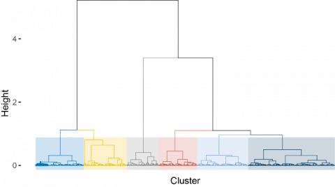
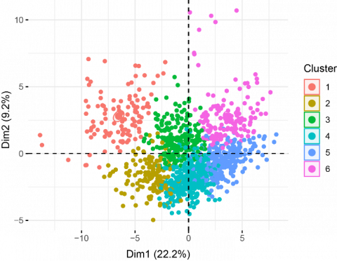
The results of the PCA analysis are shown in Figures 4 (a, b). The first ten principal dimensions explained the 74% of the variability of data. The variables that mainly contribute to the definition of each dimensions have been evaluated and compared to remove the one that are less influent in all the principal components. Of the 50 input variables, 9 variables were discarded because their contribution was assessed as uninfluential. The Figure 4a represents the cluster dendrogram of PCA: according to the characteristics expressed by the selected variables, the outcome observations can be subdivided in several groups; cutting off at the height of 1.0 six homogeneous groups (cluster) were obtained. The coloured points in the score plot (Figure 4b) represents observations of the six clusters depending on their eigenvalues for the first two principal dimensions: the nearest the points the more similar are the energy consumption observed.
The belonging to clusters has been coded as a factor variable to be included in further analysis.
Figure 3. Correlation matrix
(a)
(b)
Figure 4. Cluster dendrogram (a) and score plot (b)
5.4 Multiple linear regression models
The model was assessed on the observations referring to 2015, selected as the most recent year whose observations can be compared with those of consecutive years.
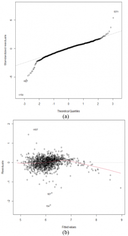
Figure 5. First model: Probability graph (a) and variance distribution of residuals (b)
The initial model (41 variables, AIC = 347.30) has a R2 value of 0.7469 and an adjusted R2 value of 0.7378, showing that the selected variables can explain the 74% of the variance in the annual electric consumption of municipalities. Table 4 shows the information on variables and their respective values for the standard error, t value and their variance inflation factor; 9 variables do not satisfy this latter criterion.
In Figures 5(a,b) are reported the results about analysis of residuals for this first model: the probability graph (Figure 5a) shows that errors are not normally distributed. The scatterplot in Figure 5b exposed a pattern, meaning that the variance of residuals tends to increase with an increasing of the predicted value. The Breusch–Pagan test evidences that the residuals are heteroskedastic (p-value < 0.001).
Figure 6. Second model: Probability graph (a) and Outliers and leverage diagnostic graph (b)
As the assumptions of a multiple lineal regression analysis were rejected, transformations on the independent variables were performed. Education degree, Family members, Age and Building Construction Year (Bcy) were redefined as explained in paragraph 4.5, becoming respectively EDU, FAM, AGE and BCY. Ten variables (HDD, Ptot, Density, EDU, FAM, AGE, inc_Taxp, Od, Avg. area of Od and BCY) were normalized according to Eq. (7); then other ten variables were created by squaring the previous ones.
Table 4. First model information
|
Variable |
Parameter Estimate |
Standard Error |
T Value |
Pr > |T| |
VIF |
|
Intercept |
8.73e+00 |
1.73e+00 |
5.031 |
<0.0001 |
- |
|
HDD |
-8.99e-05 |
3.88e-05 |
-2.313 |
0.020 |
1.79 |
|
Total Population (Ptot) |
-5.96e-04 |
1.61e-04 |
-3.695 |
<0.0001 |
122.41 |
|
Density |
1.13e-05 |
5.71e-05 |
0.200 |
0.841 |
1.77 |
|
Age 0-19 (% on Ptot) |
8.64e-01 |
5.94e-01 |
1.455 |
0.145 |
2.39 |
|
Age 20-69 (% on Ptot) |
-5.45e-02 |
4.46e-01 |
-0.122 |
0.902 |
1.79 |
|
University degree (% Ptot) |
2.33e-04 |
2.35e-04 |
0.989 |
0.322 |
17.98 |
|
Sr.H.S. Diploma (%Ptot) |
6.41e-04 |
2.05e-04 |
3.115 |
0.0018 |
45.05 |
|
Jr.H.S. Diploma (%Ptot) |
5.21e-04 |
2.63e-04 |
1.981 |
0.047 |
60.39 |
|
Primary Diploma (%Ptot) |
1.30e-03 |
2.01e-04 |
6.445 |
<0.0001 |
29.45 |
|
WorkForce (W- %Ptot) |
-9.90e-02 |
3.02e-01 |
-0.327 |
0.743 |
1.91 |
|
Employment rate (%Wtot) |
-8.27e-02 |
4.04e-01 |
-0.205 |
0.837 |
1.09 |
|
Homeworker (% on NoW) |
3.37e-01 |
3.65e-01 |
0.923 |
0.356 |
2.09 |
|
Students (% on NoW) |
8.76e-01 |
4.73e-01 |
1.849 |
0.064 |
2.00 |
|
Fixed income (% on NoW) |
-4.36e-01 |
2.94e-01 |
-1.486 |
0.137 |
2.64 |
|
Taxpayers Incavg,y(inc_Taxp) |
4.24e-05 |
3.78e-06 |
11.24 |
<0.0001 |
1.51 |
|
Fam of 1 member (%Ftot) |
-4.29e+00 |
1.51e+00 |
-2.836 |
0.004 |
19.38 |
|
Fam of 2 member (%Ftot) |
-3.45e+00 |
1.52e+00 |
-2.271 |
0.023 |
7.68 |
|
Fam of 3 member (%Ftot) |
-3.76e+00 |
1.55e+00 |
-2.424 |
0.015 |
8.06 |
|
Fam of 4 member (%Ftot) |
-3.27e+00 |
4.54e+00 |
-2.116 |
0.034 |
7.16 |
|
Fam of 5 member (%Ftot) |
-4.97e+00 |
1.81e+00 |
-2.739 |
0.006 |
2.93 |
|
Occupied dw. (tot Od) |
4.32e-05 |
1.10e-04 |
0.390 |
0.696 |
36.33 |
|
Occupied dw. (%RESb) |
7.35e-02 |
7.85e-02 |
0.936 |
0.349 |
2.24 |
|
Avg. Area of Od (supm_Od) |
-5.47e-03 |
9.08e-04 |
-6.030 |
<0.0001 |
1.68 |
|
Bcy < 1918 |
8.51e-01 |
4.20e-01 |
2.024 |
0.043 |
11.2 |
|
1919< Bcy < 1945 |
1.01e+00 |
4.27e-01 |
2.379 |
0.017 |
6.21 |
|
1946< Bcy < 1960 |
8.14e-01 |
4.40e-01 |
1.847 |
0.065 |
4.19 |
|
1961< Bcy < 1970 |
1.21e+00 |
4.54e-01 |
2.668 |
0.007 |
3.60 |
|
1971< Bcy < 1980 |
1.28e+00 |
4.55e-01 |
2.829 |
0.004 |
3.82 |
|
1981< Bcy < 1990 |
9.70e-01 |
4.97e-01 |
1.952 |
0.051 |
2.73 |
|
1991< Bcy <2000 |
1.13e-01 |
5.36e-01 |
0.211 |
0.832 |
2.45 |
|
2001< Bcy < 2005 |
1.91e+00 |
7.46e-01 |
2.561 |
0.010 |
2.42 |
|
2 Floors (%on RESb) |
2.78e-02 |
9.27e-02 |
0.300 |
0.764 |
1.99 |
|
3 Floors (%on RESb) |
1.41e-01 |
1.02e-01 |
1.374 |
0.169 |
1.90 |
|
Optimal BMS (% RESb) |
1.95e-01 |
4.22e-01 |
0.463 |
0.643 |
10.01 |
|
Good BMS (% RESb) |
1.29e-01 |
4.14e-01 |
0.312 |
0.755 |
8.26 |
|
Bad BMS (% RESb) |
-6.90e-03 |
4.76e-01 |
-0.014 |
0.988 |
6.04 |
|
Cluster 1 (ref.) |
- |
- |
- |
- |
1.45 |
|
Cluster 2 |
-2.76e-02 |
4.76e-02 |
-0.580 |
0.561 |
1.45 |
|
Cluster 3 |
7.08e-03 |
4.83e-02 |
0.146 |
0.883 |
1.45 |
|
Cluster 4 |
8.06e-03 |
5.69e-02 |
0.142 |
0.887 |
1.45 |
|
Cluster 5 |
-6.69e-03 |
6.61e-02 |
-0.101 |
0.919 |
1.45 |
|
Cluster 6 |
1.20e-01 |
6.55e-02 |
1.836 |
0.066 |
1.45 |
Note 1. HDD=Heating Degree Days; Ptot = Total population; Age=people age; H.S.=High School; NoW= No Workforce people; Fam= number of families; Ftot= Total families; Od= Occupied dwellings; BCY= Building Construction Year (% on total number of residential buildings- RESb); BMS= Building Maintenance Status.
A new initial model (55 variables) has been identified and the stepwise method was performed. The resulting model (second model) consisted in 18 variables and it has a R2 value of 0.7644 and an adjusted R2 value of 0.7607; the selected variables can explain the 76% of the variance. In Table 5 are reported the values for the standard error, t value and VIF of the selected variables. The results of residuals analysis for the second model are displayed in Figures 6(a,b). Looking at the probability graph (Figure 6a), the residuals cannot be considered as normally distributed. The variance of the residuals is not constant, going against to homoscedasticity assumption, confirmed by both the Breusch–Pagan and White test (p-value < 0.001). Considering the results of the outliers and leverage diagnostic graph (Figure 6b) a cut off at 2 times the standard deviation for both leverage and studentized residuals has been used and 68 observations (5.7% of total observations) that represent influential points were eliminated from the database.
The stepwise method resulted in an improvement in comparison to the previous models. The third model (17 variables) achieves a R2 of 0.8909 and an Adj R2 of 0.8892, other information is reported in Table 6. Variables have an acceptable VIF, therefore there is not multicollinearity.
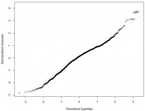
Figures 7 displays probability graph of residuals: it shows a better result, although their distribution is not normal and there are still some difficulties for predicting highest and lowest values. The results of the Breusch–Pagan and the White test still does not accept the null hypothesis of having homoscedastic residuals (p-value <0.0001).
Figure 7. Third model: Probability graph of residuals
Figure 8. Last model: variance distribution of residuals
Table 5. Second model information
|
Variable |
Parameter Estimate |
Standard Error |
T Value |
Pr > |T| |
VIF |
|
Intercept |
6.45e+00 |
1.13e-01 |
56.88 |
<0.0001 |
- |
|
nHDD |
-1.51e+01 |
5.57e+00 |
-2.70 |
0.006 |
3.91 |
|
nHDD2 |
1.07e+03+06 |
5.52e+02 |
1.94 |
0.051 |
2.48 |
|
nPtot2 |
-1.61e+00 |
9.94e+04 |
-16.22 |
<0.0001 |
5.54 |
|
nDens |
7.60e+02 |
5.07e+00 |
1.49 |
0.134 |
7.18 |
|
nDens2 |
-3.94e-02 |
1.48e+02 |
-2.65 |
0.008 |
4.35 |
|
nEDU |
-1.21e-03 |
7.71e-03 |
-1.57 |
0.116 |
2.93 |
|
n.EDU2 |
-6.66e-01 |
1.56e-03 |
-4.27 |
<0.0001 |
1.17 |
|
Students (% on NoW) |
5.84e-01 |
3.70e-01 |
1.57 |
0.114 |
2.70 |
|
Fixed income (% on NoW) |
-6.21e+01 |
1.45e-01 |
-4.28 |
<0.0001 |
1.87 |
|
Taxpayers Incavg,y(inc_Taxp) |
3.88e+02 |
4.00e+01 |
9.70 |
<0.0001 |
2.69 |
|
nFAM |
1.40e-02 |
3.68e-03 |
3.82 |
<0.0001 |
4.2 |
|
nFAM2 |
-8.22e-04 |
3.22e-04 |
-2.55 |
0.010 |
1.69 |
|
nOd |
1.39e+03 |
5.71e+01 |
24.49 |
<0.0001 |
8.14 |
|
nsupm_Od |
-7.94e-01 |
1.88e-01 |
-4.22 |
<0.0001 |
2.76 |
|
nBCY |
-2.73e-01 |
1.29e-01 |
-2.11 |
0.034 |
1.89 |
|
nBCY2 |
-3.14e+00 |
1.01e+00 |
-3.10 |
0.002 |
1.19 |
|
3 Floors (%on RESb) |
1.39e-01 |
5.84e-02 |
2.38 |
0.017 |
1.28 |
|
Optimal BMS (% RESb) |
7.80e-02 |
4.39e-02 |
1.77 |
0.076 |
1.19 |
Table 6. Third model information
|
Variable |
Parameter Estimate |
Standard Error |
T Value |
Pr > |T0.505| |
VIF |
|
Intercept |
6.53e+00 |
7.05e-02 |
92.62 |
<0.0001 |
- |
|
nHDD |
-7.41e+00 |
3.52e+00 |
-2.10 |
0.035 |
3.33 |
|
nHDD2 |
-1.15e+03 |
4.59e+02 |
2.50 |
0.012 |
2.16 |
|
nPtot2 |
8.51e+06 |
3.10e+05 |
-27.38 |
<0.0001 |
5.00 |
|
nDens |
-4.36e+00 |
4.31e+00 |
-1.01 |
0.311 |
6.72 |
|
nDens2 |
-3.23e+02 |
2.68e+02 |
-1.23 |
0.215 |
3.89 |
|
n.EDU2 |
-7.06e-03 |
1.28e-03 |
-5.49 |
<0.0001 |
1.14 |
|
Students (% on NoW) |
1.51e-01 |
2.26e-01 |
0.66 |
0.505 |
2.46 |
|
Fixed income (% on NoW) |
-4.53e-01 |
8.80e-02 |
-5.15 |
<0.0001 |
1.62 |
|
Taxpayers Incavg,y(inc_Taxp) |
3.00e+02 |
2.19e+01 |
13.68 |
<0.0001 |
1.94 |
|
nFAM |
1.34e-02 |
2.14e-03 |
6.24 |
<0.0001 |
3.47 |
|
nFAM2 |
-1.50e-03 |
2.16e-04 |
-6.95 |
<0.0001 |
1.62 |
|
nOd |
2.63e+03 |
6.29e+01 |
41.84 |
<0.0001 |
7.73 |
|
nsupm_Od |
-4.87e-01 |
1.15e-01 |
-4.23 |
<0.0001 |
2.45 |
|
nBCY |
-1.07e-01 |
8.10e-02 |
-1.32 |
0.186 |
1.85 |
|
nBCY2 |
-9.93e-01 |
6.42e-01 |
-1.54 |
0.122 |
1.20 |
|
3 Floors (%on RESb) |
5.63e-02 |
3.69e-02 |
1.52 |
0.127 |
1.30 |
|
Optimal BMS (% RESb) |
5.97e-02 |
2.80e-02 |
2.12 |
0.033 |
1.17 |
Table 7. Last model information
|
Variable |
Parameter Estimate |
Standard Error |
T Value |
Pr > |T| |
VIF |
|
Intercept |
6.53e+00 |
7.62e-02 |
85.65 |
<0.0001 |
- |
|
nHDD |
-7.41e+00 |
3.46e+00 |
-2.13 |
0.032 |
3.33 |
|
nHDD2 |
1.15e+03 |
5.33e+02 |
2.15 |
0.031 |
2.16 |
|
nPtot2 |
-8.51e+06 |
5.63e+05 |
-15.11 |
<0.0001 |
5.00 |
|
nDens |
-4.36e+00 |
3.73e+00 |
-1.16 |
0.242 |
6.72 |
|
nDens2 |
-3.32e+02 |
2.29e+02 |
-1.44 |
0.147 |
3.89 |
|
n.EDU2 |
-7.06e-03 |
1.46e-03 |
-4.82 |
<0.0001 |
1.14 |
|
Students (% on NoW) |
1.51e-01 |
2.49e-01 |
0.60 |
0.544 |
2.46 |
|
Fixed income (% on NoW) |
-4.53e-01 |
9.94e-02 |
-4.56 |
<0.0001 |
1.62 |
|
Taxpayers Incavg,y(inc_Taxp) |
3.00e+02 |
2.51e+01 |
11.93 |
<0.0001 |
1.94 |
|
nFAM |
1.34e-02 |
2.33e-03 |
5.73 |
<0.0001 |
3.47 |
|
nFAM2 |
-1.50e-03 |
2.48e-04 |
-6.06 |
<0.0001 |
1.62 |
|
nOd |
2.63e+03 |
8.03e+01 |
32.81 |
<0.0001 |
7.73 |
|
nsupm_Od |
-4.87e-01 |
1.17e-01 |
-4.15 |
<0.0001 |
2.45 |
|
nBCY |
-1.07e-01 |
8.44e-02 |
-1.26 |
0.204 |
1.85 |
|
nBCY2 |
-9.93e-01 |
6.10e-01 |
-1.62 |
0.103 |
1.20 |
|
3 Floors (%on RESb) |
5.63e-02 |
3.90e-02 |
1.44 |
0.149 |
1.30 |
|
Optimal BMS (% RESb) |
5.97e-02 |
2.77e-02 |
2.15 |
0.031 |
1.17 |
Finally, a more stable model was found with uncorrelated independent variables and all other assumptions achieved. The last model counts of 17 variables whit both linear and quadratic predictors. Table 7 present the information about the last model, Table 8 reports values of R2 and Adj R2 comparing all the model evaluated in this study. The scatterplot in Figure 8 shows an acceptable distribution of the variance of residuals if we consider the different scale on the y-axis with respect to Figure 5; the presence of a quadratic trend has been adjusted with the White correction.
Table 8. Value of R2 and Adj-R2 of the evaluated models
|
|
R2 |
Adj R2 |
|
First model |
0.7469 |
0.7378 |
|
Second model |
0.7644 |
0.7607 |
|
Third model |
0.8909 |
0.8892 |
|
Last model |
0.8909 |
0.8892 |
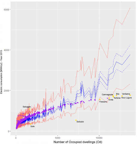
To verify the validity of the last predicting model, the observed values of the annual electricity consumption of the 1186 municipalities have been observed in comparison to the graph representing the confidence and prediction interval of the last model. This check has been done for all the six years whose data were available. Figure 9 reports the results for the observed values (violet points) referred to the year 2015, in relation to the number of occupied dwellings. As shown in Figures 9, only few observed values (59 observations, 5 %) fall outside the prediction interval, and some of them (yellow points) are highlighted and named, this sustain the capacity of the model to predict annual electric energy consumption of municipalities except for very small (e.g. Sale, Saluggia) or large ones (e.g. Verbania, Novi Ligure, Bra). The observed values that the model cannot predicted have been identified and descripted in Table 9 according to some significant variables. For each of the six years is reported the total number of observed values that cannot be predicted by the model, the main statistical parameters about their electric consumption and their total population, and the number of observations for each cluster.
Table 9. Description of the observed values outside the prediction interval of the predicting model
|
Year |
N. |
Electric Consumption [MWh/yr] |
Total Population [n] |
Cluster |
|||||||||
|
|
|
Min |
Max |
Median |
Min |
Max |
Median |
1 |
2 |
3 |
4 |
5 |
6 |
|
2010 |
59 |
71,268 |
32,242,421 |
489,058 |
52 |
25,986 |
350 |
21 |
13 |
7 |
4 |
6 |
8 |
|
2012 |
57 |
72,074 |
30,783,835 |
332,997 |
52 |
25,986 |
323 |
19 |
15 |
7 |
4 |
5 |
7 |
|
2013 |
59 |
71,255 |
30,183,758 |
316,550 |
52 |
25,986 |
323 |
21 |
14 |
7 |
4 |
5 |
8 |
|
2014 |
60 |
70,938 |
28,586,741 |
281,745 |
52 |
25,986 |
251 |
18 |
14 |
6 |
6 |
6 |
10 |
|
2015 |
62 |
70,959 |
39,169,077 |
317,418 |
52 |
25,986 |
326 |
17 |
13 |
6 |
9 |
6 |
11 |
|
2016 |
61 |
67,692 |
28,433,423 |
257,178 |
52 |
25,986 |
250 |
16 |
13 |
8 |
8 |
6 |
10 |
The model for predicting the residential annual electric consumption at municipal scale points out that the most influential variables comprehend climatic-environmental, socio-economic, and building characteristics. Regarding to the climatic features the model evidences that the HDD is associated with an increase on energy consumption, as the population density, but these variables does not show a stronger influence. The number of total population and the occupied dwellings is positively correlated and significantly predicting. About the socio-economic variables, the most significant variables are the education degree, the yearly average income, and the average number of members in a family. Also, the number of students and owners of fixed income shows a stronger influence on energy consumptions, the first is positively correlated but less significant, while the second is negatively correlated and very significant.
Regarding to the building geometry, the average surface of occupied dwellings is significant, but at contrary is negatively correlated with the electric consumption, as it is for the average age of buildings.
Figure 9. Observed values of electricity consumption of 2015 inside (violet points) and outside (yellow points) the confidence (blue lines) and prediction (red lines) intervals.
In conclusion, the resulted models evidenced the most important variables that affect the electric consumption of residential users depends on the characteristics of the building itself but also on the characteristics of the socio-economic environment of each municipality.
The model can predict consumption in the majority of municipalities, with the exception of very small and very large municipalities. It has to be considered that in 2018 a regional administrative reorganization brought together about 80 municipalities considered too small. Metropolitan cities and densely populated municipalities require different assessments.
The statistical methodology used in this study could be used for evaluating the energy consumption at municipal scale in another Italian region, starting from the available ISTAT databases. It can support urban planners and decisions makers for evaluating energy consumption at territorial scale and contribute identifying possible aggregation of neighbouring municipalities interested in creating Energy Communities.
The methodology presented in this work can implemented and used in evaluating variables that influenced electric consumption of other energy users involved in the EC: municipal buildings and service and companies.
[1] European Commission (2012). Energy Roadmap 2050, Publications Office of the European Union, Luxembourg. https://doi.org/10.2833/10759
[2] Fumo N., Biswas M.A.R. (2015). Regression analysis for prediction of residential energy consumption. Renewable and Sustainable Energy Reviews, 47: 332-343. http://dx.doi.org/10.1016/j.rser.2015.03.035
[3] Swan, L.G., Ugursal, I.V. (2009). Modelling of end-use energy consumption in the residential sector: A review of modelling techniques. Renewable and Sustainable Energy Reviews, 13: 1819-1835. https://doi.org/10.1016/j.rser.2008.09.033
[4] Renewable self-consumers and energy communities. (2017). Council of European Energy Regulators.
[5] Frieden, D., Tuerk, A., Roberts J., D’Herbermont, S., Gubina, A. (2019). Collective self-consumption and energy communities: Overview of emerging regulatory approaches in Europe. 2019 16th International Conference on the European Energy Market, Ljubljana, Slovenia, pp. 1-6. https://dx.doi.org/10.1109/EEM.2019.8916222
[6] Bukovszki, V., Magyari, A., Braun, M.K., Pardi, K., Reith, A. (2020). Energy modelling as a trigger for energy communities: A joint socio-technical perspective. Energies, 13(9): 2274. https://doi.org/10.3390/en13092274
[7] Mutani, G., Todeschi, V., Tartaglia, A., Nuvoli, G. (2018). Energy communities in piedmont region. The case study in Pinerolo territory. 2018 IEEE International Telecommunications Energy Conference (INTELEC), Turin, Italy, pp. 1-8. https://doi.org/10.1109/INTLEC.2018.8612427
[8] Olofsson T., Andersson S. and Sjögren J.U. (2009). Building energy parameter investigations based on multivariate analysis. Energy and Buildings, 41(1): 71-80. https://doi.org/10.1016/j.enbuild.2008.07.012
[9] Howard B., Parshall L., Thompson J., Hammer S., Dickinson J., Modi V. (2012). Spatial distribution of urban building energy consumption by end use. Energy and Buildings, 45: 141-151. https://doi.org/10.1016/j.enbuild.2011.10.061
[10] Mastrucci, A., Baume, O., Stazi F., Leopold, U. (2014). Estimating energy savings for the residential building stock of an entire city: A GIS-based statistical downscaling approach applied to Rotterdam. Energy and Buildings, 75: 358-367. https://doi.org/10.1016/j.enbuild.2014.02.032
[11] Nouvel, R., Mastrucci, A., Leopold, U., Baume, O., Coors, V., Eicker, U. (2015). Combining GIS-based statistical and engineering urban heat consumption models: Towards a new framework for multi-scale policy support. Energy and Buildings, 107: 204-212. https://doi.org/10.1016/j.enbuild.2015.08.021
[12] Mutani, G., Fontana, R., Barreto, A. (2019). Statistical GIS-based analysis of energy consumption for residential buildings in Turin (IT). IEEE CANDO EPE 2019 Conference, Budapest, Hungary, pp. 179-184, https://doi.org/10.1109/CANDO-EPE47959.2019.9111035
[13] Chen, J., Wang, X., Steemers, K. (2013). A statistical analysis of a residential energy consumption survey study in Hangzhou, China. Energy Build, 66: 193-202. https://doi.org/10.1016/j.enbuild.2013.07.045
[14] Bianco, V., Manca, O., Nardini, S. (2013). Linear regression models to forecast electricity consumption in Italy. Energy Sources Part B, 8: 86-93. https://doi.org/10.1080/15567240903289549
[15] Gans, W., Alberini, A., Longo, A. (2013). Smart meter devices and the effect of feedback on residential electricity consumption: Evidence from a natural Experiment in Northern Ireland. Energy Economics, 36: 729-743.
[16] Nie, H., Kemp, R. (2010). Index decomposition analysis of residential energy consumption in China: 2002-2010. Applied Energy, 121: 10-19. https://doi.org/10.1016/j.apenergy.2014.01.070
[17] Regione Piemonte, Geoportale Piemonte, http://www.geoportale.piemonte.it/cms, accessed on May 25th, 2020.
[18] National Institute of Statistic (in Italian, Istituto Nazionale di Statistica ISTAT), Population and Housing Census, updated to 2011, http://daticensimentopopolazione.istat.it/Index.aspx?lang=it, accessed on May 25th, 2020.
[19] Mutani, G., Gabrielli, C., Nuvoli, G. (2020). Energy performance certificates analysis in Piedmont Region (IT). A new oil field never exploited has been discovered. Italian Journal of Engineering Science, 64(1): 71-82. https://doi.org/10.18280/ti-ijes.640112
[20] Moghadam S.T, Toniolo, J., Mutani, G., Lombardi, P. (2018). A GIS-statistical approach for assessing built environment energy use at urban scale. Sustainable Cities and Society, 37: 70-84. https://doi.org/10.1016/j.scs.2017.10.002
[21] Mutani, G., Fontanive, M., Arboit, M.E. (2018). Energy-use modelling for residential buildings in the metropolitan area of Gran Mendoza (AR). Italian Journal of Engineering Science, 62(2). https://doi.org/10.18280/ti-ijes.620204
[22] Mutani, G., Beltramino, S., Forte, A. (2020). A clean energy atlas for energy communities in Piedmont Region (Italy). International Journal of Design & Nature and Ecodynamics, 15(3): 343-353. https://doi.org/10.18280/ijdne.150308
[23] Ricci, V. (2006). Principali tecniche di regressione con R Copyright 2006. https://cran.r-project.org/doc/contrib/Ricci-regression-it.pdf, accessed on May 25th, 2020.
[24] White, H. (1980). A heteroskedasticity-consistent covariance matrix estimator and a direct test for heteroskedasticity. Econometrica, 48: 817-838. https://doi.org/10.2307/1912934