OPEN ACCESS
In the present study, analytical solutions have been developed for two-dimensional solute transport in steady field of groundwater flow with different longitudinal and lateral dispersion coefficients in semi-infinite heterogeneous porous medium for a varying type input point source. Dispersion coefficient is considered squarely proportional to the groundwater velocity along both longitudinal and lateral directions while groundwater velocity is considered linear spatially dependent function in both directions. The flow is assumed to be two-dimensional in a horizontal plane and the nature of pollutant and porous medium are considered chemically non-reactive. The geological formation is initially not solute free. Varying type input condition for multiple point sources through arbitrary time-dependent function is considered at origin. Concentration gradient is considered zero at infinity. New space variables are introduced by certain transformations to get the analytical solutions. The solutions in the real time domain are obtained by using Laplace Integral Transform Technique. The obtained analytical solutions are illustrated graphically to study the effect of various parameters on the solute transport in various time domains for spatially dependent velocity.
advection, dispersion, unit step function, point source, Laplace integral transform, heterogeneous medium
A wide variety of analytical models describing groundwater flow and solute transport in porous media have been developed in the last two-three decades. Analytical solutions for aquifers have been developed for several types of boundary conditions for a finite and semi-infinite domain. The majority of analytical solutions developed on transport issue from several stand points or hypothesis in one, two and three-dimensional groundwater flow in aquifers with common assumptions, constant porosity, steady and unsteady pore-water velocity with or without retardation factor. Retardation factor is one of the major processes affecting the contaminants dissolved in groundwater. In real scenario, most of the geological formations are heterogeneous in nature which originates from the variability of the hydraulic conductivity. Groundwater velocity and hydrodynamic dispersion coefficient are key parameters for description of any solute transport phenomena in porous media. Solute transport in soil, reservoir and aquifer is generally governed by advection-dispersion equation which is a parabolic partial differential equation of second order. In subsurface, groundwater velocity and flow direction are functions of the hydraulic gradient, which may vary with time and space. In general, spreading of pollutant causes due to gradient magnitude variability and gradient direction variability [1].
Magnitudes of contaminant dispersivity have direct relation with distance from the contaminant source [2]. Cirpka and Kitanidis [3] demonstrated that transport distance and vertical discharge rate are closely related with dispersivities. Watson and Jones [4] obtained analytical solution with velocity dependent dispersion. Variation in hydraulic gradient in terms of direction is more important than magnitude variation in hydraulic gradient was discussed by Goode and Konikow [5]. Watson et al. [6] observed that the hydrodynamic dispersion coefficient and seepage velocity are related with non-linearly to each other. Qiu et al. [7] obtained an analytical solution for solute transport model with spatially dependent flow velocity and solute dispersion using generalized integral transform technique. Guerrero et al. [8] derived an analytical solution of advection dispersion equation using Integral transform technique with first order decay term for multi-layered media. You and Zhan [9] developed semi-analytical solutions for one-dimensional solute transport in a finite domain with time-dependent sources and distance dependent dispersivities.
Singh et al. [10] obtained analytical solutions for one-dimensional solute dispersion with uniform and time varying dispersion in a semi-infinite aquifer using the Laplace transform technique. Falta and Wang [11] presented a semi-analytical solution of one-dimensional advection-dispersion equation with matrix diffusion process by assuming the low permeability in semi-infinite domain. Yadav and Kumar [12] established a mathematical model for two-dimensional solute transport in a semi-infinite heterogeneous porous medium with spatially and temporally dependent coefficients for pulse type input concentration of varying nature. Das et al. [13] presented analytical and numerical solutions for conservative solute transport modeling in homogeneous semi-infinite porous medium. Yadav and Kumar [14] established an analytical solution for two-dimensional advection dispersion equation for conservative solute transport in a semi-infinite heterogeneous porous medium with pulse type input point source of uniform nature. In real situations, two-dimensional contaminant transport models are more advantageous in comparison to one-dimensional models because they can be responsible for concentration gradients and contaminant transport in directions perpendicular to the groundwater flow. The majority of the available analytical solutions of conservative solutes are derived by solving only single point source.
The objective of the present study is to develop an analytical solution for advection-dispersion equation in a two-dimensional heterogeneous semi-infinite porous medium using the Laplace Integral Transformation Technique (LITT). The heterogeneity of the medium is expressed by spatially dependent flow which causes due to variation in velocity of the flow through it. Solute transport phenomenon takes place in the direction of flow. Three main assumptions behind the proposed model are (i) multiple point source (ii) groundwater velocity linear spatially dependent function (iii) dispersion coefficient is squarely proportional to groundwater velocity. The medium is supposed to have a uniform solute concentration before an injection of pollutant in domain. Concentration gradients are considered zero at infinity along both longitudinal and lateral boundaries. The graphical illustrations along with its physical interpretations are also discussed.
The geological formation is assumed heterogeneous and semi-infinite along both x and y directions. In developing the analytical solution, it assumed that solute is conservative and transport through porous medium in two-dimension which is described by second order partial differential equation of parabolic type, generally known as advection-dispersion equation [2, 15].
$\frac{\partial C}{\partial t}=\frac{\partial}{\partial x}\left(D_{x} \frac{\partial C}{\partial x}-u C\right)+\frac{\partial}{\partial y}\left(D_{y} \frac{\partial C}{\partial y}-v C\right)$ (1)
where, $C\left[\mathrm{ML}^{-3}\right]$ represents the solute concentration of the pollutant transporting along the flow field through the medium at a position $(x[L], y[L])$ and time $t[T]$. $D_{x}\left[\mathrm{L}^{2} \mathrm{T}^{-1}\right]$ and $D_{y}\left[\mathrm{L}^{2} \mathrm{T}^{-1}\right]$ are the longitudinal and lateral dispersion coefficients, respectively. $u\left[\mathrm{LT}^{-1}\right]$ and $v\left[\mathrm{LT}^{-1}\right]$ are the unsteady uniform groundwater velocity along longitudinal and lateral directions, respectively. First term on the left hand side of the Eq. (1) is represent change in concentration with time in liquid phase. First and third terms on the right-hand side of the Eq.(1) describe the influence of the dispersion on the concentration distribution in longitudinal and lateral directions, respectively while second and fourth terms on the right-hand side of the Eq.(1) describe the change of the concentration due to advective transport in longitudinal and lateral directions, respectively. The effect of molecular diffusion is not taken into account due to dominance of the mechanical dispersion on the hydrodynamic dispersion during solute transport. The medium is supposed to have a uniform solute concentration $C_{i}$ before an injection of pollutant in the domain. The input condition is considered of varying type. The right boundary is assumed that of flux type homogeneous condition at far ends of the domain along both the longitudinal and lateral directions. Van Genuchten and Alves [16] prompted that the Cauchy’s boundary is more realistic than the Dirichlet’s boundary. This type phenomenon may be formulate mathematically as:
$C(x, y, t)=C_{i} \quad ; \quad t=0, x \geq 0, y \geq 0$ (2)
$-D_{x} \frac{\partial C}{\partial x}+u C=u C_{0}\left(p t^{2}+q t+r\right)$
$\left[u\left(t-t_{1}\right)-u\left(t-t_{2}\right)\right] ; x=0, t>0$ (3.a)
$-D_{y} \frac{\partial C}{\partial y}+v C=v C_{0}\left(p t^{2}+q t+r\right)$
$\left[u\left(t-t_{1}\right)-u\left(t-t_{2}\right)\right] ; \quad y=0, t>0$ (3.b)
$\frac{\partial C(x, y, t)}{\partial x}=0, \frac{\partial C(x, y, t)}{\partial y}=0 ; t \geq 0, x \rightarrow \infty, y \rightarrow \infty$ (4)
where, $C_{0}$ is the reference concentration, p, q and r are parameters of the quadratic function of time in pulse type boundary conditions at $x=0, y=0$. t1 and t2 are the beginning and end times of the source activation, respectively. $u\left(t-t_{i}\right)$ being the Heaviside function defined to be 0 for $t<t_{i}$ and 1 for $t \geq t_{i}$. Pollutants fabrications on the surface reach at a point uniformly and are filtered down the stream. As soon as the pollutant reach due to infiltration from a point source occurring on the surface. It may treat that as source; hence the input concentration increases in interval of time and once it is eliminated, the input starts decreasing instead of becomes zero at once. This situation may be defined by a mixed type input condition which is given by Eq. (3a, b). Eq. (3) is depicted in following Figure 1 given below.
Figure 1. Depiction of the input boundary condition
Dispersion coefficient is considered proportional to square of the space variable and groundwater flow is supposed to vary linearly to space variable [17]. In this study, dispersion coefficient along both longitudinal and lateral directions are considered as squarely proportional to corresponding groundwater velocity in that direction, respectively while groundwater velocity along both longitudinal and lateral directions are supposed to vary linearly to the corresponding space variable, respectively. They are mathematically defined as:
$\left.\begin{array}{l}u=u_{0}(1+a x) \text { and } D_{x} \propto u^{2} \Rightarrow D_{x}=D_{x_{0}}(1+a x)^{2} \\ v=v_{0}(1+a y) \text { and } D_{y} \propto v^{2} \Rightarrow D_{y}=D_{y_{0}}(1+a y)^{2}\end{array}\right\}$ (5)
where, $a\left[L^{-1}\right]$ is the heterogeneous parameter along both longitudinal and lateral directions and have dimension inverse of space variable [18]. Heterogeneity of the porous medium means the transport properties like porosity or hydraulic conductivity is not uniform throughout the domain but depends upon the position. $\mathrm{D}_{\mathrm{x}_{0}}, \mathrm{D}_{\mathrm{y}_{0}}, u_{0}$ and $v_{0}$ are initial dispersion coefficient and unsteady uniform pore groundwater velocity along longitudinal and lateral directions, respectively.
Substituting the values from Eq. (5) in Eq. (1), we have
$\begin{align} & \frac{\partial C}{\partial t}=\frac{\partial }{\partial x}\left\{ {{D}_{{{x}_{0}}}}{{\left( 1+a\,x \right)}^{2}}\frac{\partial C}{\partial x}-{{u}_{0}}\left( 1+a\,x \right)\,C \right\} \\ & \,\,\,\,\,\,\,\,\,\,\,\,+\frac{\partial }{\partial y}\left\{ {{D}_{{{y}_{0}}}}{{\left( 1+a\,y \right)}^{2}}\frac{\partial C}{\partial y}-{{v}_{0}}\left( 1+a\,y \right)\,C \right\} \\ \end{align}$ (6)
With the help of Eq. (5), the initial and boundary conditions in Eqns. (2-4) may be written as:
$C(x,y,t)={{C}_{i}}\,\,\,\,\,\,\,\,\,\,\,;\,\,\,\,t=0\,\,,\,\,\,x\ge 0\,\,,\,\,y\ge 0$ (7)
$\begin{align} & -{{D}_{{{x}_{0}}}}\frac{\partial C}{\partial x}+{{u}_{0}}C={{u}_{0}}{{C}_{0}}\left( p{{t}^{2}}+qt+r \right)\, \\ & \,\,\,\,\,\,\,\,\,\,\,\,\,\,\,\,\,\,\,\,\,\,\,\,\,\,\,\,\,\,\,\,\,\,\,\,\,\left[ u\left( t-{{t}_{1}} \right)-u\left( t-{{t}_{2}} \right) \right]\,\,\,\,;\,\,x=0,t>0 \\ \end{align}$ (8.a)
$\begin{align} & -{{D}_{{{y}_{0}}}}\frac{\partial C}{\partial y}+{{v}_{0}}C={{v}_{0}}{{C}_{0}}\left( p{{t}^{2}}+qt+r \right)\, \\ & \,\,\,\,\,\,\,\,\,\,\,\,\,\,\,\,\,\,\,\,\,\,\,\,\,\,\,\,\,\,\,\,\,\,\,\,\,\left[ u\left( t-{{t}_{1}} \right)-u\left( t-{{t}_{2}} \right) \right]\,\,;\,\,y=0,\,t\,>0 \\ \end{align}$ (8.b)
$\frac{\partial C\left( x,y\,,t \right)}{\partial x}=0\,\,,\frac{\partial C\left( x,y\,,t \right)}{\partial y}=0\,;\,t\ge 0\,\,\,x\to \infty ,\,\,y\to \infty $ (9)
Let us introduce new independent space variables X and Y through the transformations (Kumar et al. [18]) defined as:
$X=\frac{\log \left( 1+a\,x \right)}{a}\,$ and $Y=\frac{\log \left( 1+a\,y \right)}{a}$ (10)
Applying transformation from Eq. (10) in Eqns. (6-9), we have
$\frac{\partial C}{\partial t}={{D}_{{{x}_{0}}}}\,\frac{{{\partial }^{2}}C}{\partial {{X}^{2}}}+{{D}_{{{y}_{0}}}}\,\frac{{{\partial }^{2}}C}{\partial {{Y}^{2}}}-{{U}_{1}}\frac{\partial C}{\partial X}-{{U}_{2}}\frac{\partial C}{\partial Y}-{{\gamma }_{0}}\,C$ (11)
$C(X,Y,t)={{C}_{i}}\,\,\,\,\,\,\,\,\,\,\,;\,\,\,\,t=0\,\,,\,\,\,X\ge 0\,,\,Y\ge 0$ (12)
$\begin{align} & -{{D}_{{{x}_{0}}}}\frac{\partial C}{\partial X}+{{u}_{0}}C={{u}_{0}}{{C}_{0}}\left( p{{t}^{2}}+qt+r \right) \\ & \,\,\,\,\,\,\,\,\,\,\,\,\,\,\,\,\,\,\,\,\,\,\,\,\,\,\,\,\,\,\,\,\,\,\,\,\,\,\,\,\left[ u\left( t-{{t}_{1}} \right)-u\left( t-{{t}_{2}} \right) \right]\,\,\,\,\,;\,X=0,\,t\,>0 \\ \end{align}$ (13.a)
$\begin{align} & -{{D}_{{{y}_{0}}}}\frac{\partial C}{\partial Y}+{{v}_{0}}C={{v}_{0}}{{C}_{0}}\left( p{{t}^{2}}+qt+r \right)\, \\ & \,\,\,\,\,\,\,\,\,\,\,\,\,\,\,\,\,\,\,\,\,\,\,\,\,\,\,\,\,\,\,\,\,\,\,\,\,\,\,\left[ u\left( t-{{t}_{1}} \right)-u\left( t-{{t}_{2}} \right) \right]\,\,\,;\,\,\,Y=0,\,t\,>0 \\ \end{align}$ (13.b)
$\frac{\partial C(X,Y,t)}{\partial X}=0\,\,,\,\,\frac{\partial C(X,Y,t)}{\partial Y}=0\,\,\,;\,t\ge 0\,\,\,X\to \infty \,\,,\,\,Y\to \infty $ (14)
where, ${{U}_{1}}=\left( {{u}_{0}}-a{{D}_{{{x}_{0}}}} \right)\,\,,\,\,{{U}_{2}}=\left( {{v}_{0}}-a{{D}_{{{y}_{0}}}} \right)\,\,,\,\,{{\gamma }_{0}}=a\,\left( {{u}_{0}}+{{v}_{0}} \right)$.
Let us introduce another new independent space variable Z through the transformation (Carnahan and Remer [19]) defined as:
$Z=X+Y$ (15)
Applying this transformation from Eq. (15) in Eqns. (11-14), we have
$\frac{\partial C}{\partial t}={{D}_{0}}\frac{{{\partial }^{2}}C}{\partial {{Z}^{2}}}-{{U}_{0}}\frac{\partial C}{\partial Z}-{{\gamma }_{0}}\,C$ (16)
$C(Z,t)={{C}_{i}}\,\,\,\,;\,\,\,t=0\,\,,\,\,\,Z\ge 0$ (17)
$\begin{align} & -{{D}_{0}}\frac{\partial C}{\partial Z}+{{w}_{0}}C={{w}_{0}}{{C}_{0}}\left( p{{t}^{2}}+qt+r \right)\, \\ & \,\,\,\,\,\,\,\,\,\,\,\,\,\,\,\,\,\,\,\,\,\,\,\,\,\,\,\,\,\left[ u\left( t-{{t}_{1}} \right)-u\left( t-{{t}_{2}} \right) \right]\,\,\,\,\,\,\,\,\,;\,\,\,\,\,\,\,\,Z=0,\,\,\,\,t\,>0 \\ \end{align}$ (18)
$\frac{\partial C(Z,t)}{\partial Z}=0\,\,\,\,\,;\,\,\,\,\,t\ge 0\,\,\,Z\to \infty $ (19)
where, ${{U}_{0}}={{u}_{0}}+{{v}_{0}}-a\left( {{D}_{{{x}_{0}}}}+{{D}_{{{y}_{0}}}} \right),$ ${{D}_{0}}=\left( {{D}_{{{x}_{0}}}}+{{D}_{{{y}_{0}}}} \right),\,\,$ $\,{{\gamma }_{0}}=a\,{{w}_{0}},$ ${{w}_{0}}=\left( {{u}_{0}}+{{v}_{0}} \right)$ .
Applying the Laplace integral transformation on the above Eqns. (16-19), it reduces into an ordinary differential equation of second order which comprises of following three equations:
${{D}_{0}}\frac{{{d}^{2}}\bar{C}}{d{{Z}^{2}}}-{{U}_{0}}\frac{d\bar{C}}{dZ}-\left( s+{{\gamma }_{0}} \right)\bar{C}=-{{C}_{i}}$ (20)
$\begin{align} & -{{D}_{0}}\frac{d\bar{C}}{dZ}+{{w}_{0}}\bar{C}={{w}_{0}}{{C}_{0}}\left[ \left( pt_{1}^{2}+q{{t}_{1}}+r \right)\frac{\exp \left( -s\,{{t}_{1}} \right)}{s} \right. \\ & +\left( 2p{{t}_{1}}+q \right)\frac{\exp \left( -s\,{{t}_{1}} \right)}{{{s}^{2}}}+2p\frac{\exp \left( -s\,{{t}_{1}} \right)}{{{s}^{3}}}-\left( pt_{2}^{2}+q{{t}_{2}}+r \right) \\ & \,\frac{\exp \left( -s\,{{t}_{2}} \right)}{s}\left. -\left( 2p{{t}_{2}}+q \right)\frac{\exp \left( -s\,{{t}_{2}} \right)}{{{s}^{2}}}-2p\frac{\exp \left( -s\,{{t}_{2}} \right)}{{{s}^{3}}} \right]\,;\,Z=0 \\ \end{align}$ (21)
$\frac{d\bar{C}}{dZ}=0\,\,\,\,\,\,\,\,\,;\,\,\,\,\,\,\,Z\to \infty $ (22)
where, $\,\bar{C}=\int_{0}^{\infty }{C(Z,t)\,{{e}^{-s\,t}}\,dt}$ and s is a Laplace parameter.
Thus, the general solution of ordinary differential Eq. (20) may be written as:
$\begin{align} & \bar{C}\left( Z,s \right)=\,{{c}_{1}}\exp \left( \mu +Z\sqrt{\alpha +\beta \,s} \right)+{{c}_{2}}\exp \left( \mu -Z\sqrt{\alpha +\beta \,s} \right) \\ & \,\,\,\,\,\,\,\,\,\,\,\,\,\,\,\,\,\,\,\,\,+\frac{{{C}_{i}}}{\left( s+{{\gamma }_{0}} \right)} \\ \end{align}$ (23)
where, $\alpha =\frac{U_{0}^{2}}{4\,D_{0}^{2}}+\frac{{{\gamma }_{0}}}{{{D}_{0}}}\,\,,\,\,\beta =\frac{1}{{{D}_{0}}}\,\,,\,\,\mu =\frac{{{U}_{0}}Z}{2\,{{D}_{0}}}$ .
Using boundary conditions Eq. (21) and Eq. (22) into Eq. (23) to eliminate arbitrary constants ${{c}_{1}}$ and ${{c}_{2}}$ , we get the particular solution of the Eq. (20) as:
$\begin{align} & \bar{C}\left( Z,s \right)=\frac{{{C}_{i}}}{\left( s+{{\gamma }_{0}} \right)}-\frac{\beta \,{{w}_{0}}{{C}_{i}}\,\exp \left( \mu -Z\sqrt{\alpha +\beta \,s} \right)}{\left( s+{{\gamma }_{0}} \right)\,\left( \sqrt{\alpha }+\sqrt{\alpha +\beta \,s} \right)}+\left\{ \left( pt_{1}^{2}+q{{t}_{1}}+r \right) \right. \\ & \,\,\,\,\,\,\,\,\,\,\,\,\,\,\,\,\,\,\,\,\,\,\,\,\,\,\,\frac{\exp \left( -s\,{{t}_{1}} \right)}{s}+\left( 2p{{t}_{1}}+q \right)\frac{\exp \left( -s\,{{t}_{1}} \right)}{{{s}^{2}}}+2p\frac{\exp \left( -s\,{{t}_{1}} \right)}{{{s}^{3}}} \\ & \,\,\,\,\,\,\,\,\,\,\,\,\,\,\,\,\,\,\,\,\,\,\,\,-\left( pt_{2}^{2}+q{{t}_{2}}+r \right)\frac{\exp \left( -s\,{{t}_{2}} \right)}{s}-\left( 2p{{t}_{2}}+q \right)\frac{\exp \left( -s\,{{t}_{2}} \right)}{{{s}^{2}}} \\ & \,\,\,\,\,\,\,\,\,\,\,\,\,\,\,\,\,\,\,\,\,\,\,\,\,\left. -2p\frac{\exp \left( -s\,{{t}_{2}} \right)}{{{s}^{3}}} \right\}\frac{\beta \,{{w}_{0}}{{C}_{0}}\exp \left( \mu -Z\sqrt{\alpha +\beta \,s} \right)}{\left( s+{{\gamma }_{0}} \right)\,\left( \sqrt{\alpha }+\sqrt{\alpha +\beta \,s} \right)} \\ \end{align}$ (24)
Now, applying Inverse Laplace integral transform on it using the appropriate tables [16, 20] and requisite transformations back, the desired analytical solution may be obtained in terms of $C(Z, t)$ as:
$C\left( Z,t \right)=\,{{C}_{i}}\exp \left( -{{\gamma }_{0}}\,t \right)-\beta \,{{w}_{0}}\,{{C}_{i}}\,F\left( Z,t \right)\,;\,\,0\,\,\le \,\,t\,\,<\,\,{{t}_{1}}$ (25)
$\begin{align} & C\left( Z,t \right)={{C}_{i}}\exp \left( -{{\gamma }_{0}}\,t \right)-\beta \,{{w}_{0}}\,{{C}_{i}}\,F(Z,t)+\beta \,{{w}_{0}}\,{{C}_{0}} \\ & \,\,\,\,\,\,\,\,\,\,\,\,\,\,\,\,\,\,\,\,\,\,\exp \left( \frac{{{U}_{0}}\,Z}{2\,{{D}_{0}}} \right)\,\left\{ \,\left( pt_{1}^{2}+q{{t}_{1}}+r \right) \right.G\left( Z,t-{{t}_{1}} \right) \\ & \,\,\left. +\left( 2p{{t}_{1}}+q \right)H\left( Z,t-{{t}_{1}} \right)+2\,p\,J\left( Z,t-{{t}_{1}} \right) \right\}\,\,\,\,\,\,\,;\,\,\,{{t}_{1}}\,\le \,\,t\,\,<\,{{t}_{2}} \\\end{align}$ (26)
$\begin{align} & C\left( Z,t \right)={{C}_{i}}\exp \left( -{{\gamma }_{0}}\,t \right)-\beta \,{{w}_{0}}\,{{C}_{i}}\,F(Z,t)+\beta \,{{w}_{0}}\,{{C}_{0}} \\ & \,\exp \left( \frac{{{U}_{0}}\,Z}{2\,{{D}_{0}}} \right)\,\left\{ \,\left( pt_{1}^{2}+q{{t}_{1}}+r \right) \right.G\left( Z,t-{{t}_{1}} \right)+\left( 2p{{t}_{1}}+q \right)H\left( Z,t-{{t}_{1}} \right) \\ & \,\,\,\,\,\,\,\,\,+2\,p\,J\left( Z,t-{{t}_{1}} \right)-\left( pt_{2}^{2}+q{{t}_{2}}+r \right)G\left( Z,t-{{t}_{2}} \right) \\ & \,\,\,\,\,\,\,\,\,\left. -\left( 2p{{t}_{2}}+q \right)H\left( Z,t-{{t}_{2}} \right)-2\,p\,J\left( Z,t-{{t}_{2}} \right)\, \right\}\,\,\,\,\,\,\,;\,\,\,\,\,\,\,t\,\ge {{t}_{2}} \\\end{align}$ (27)
where,
$\begin{align} & F\left( Z,t \right)=\frac{\exp \left( -\delta \,Z-{{\gamma }_{0}}\,t \right)}{2\,\left( \delta +\sqrt{\alpha } \right)}erfc\left( \frac{\beta \,Z-2\delta \,t}{2\,\sqrt{\beta \,t}} \right)-\frac{\exp \left( \delta \,Z-{{\gamma }_{0}}\,t \right)}{2\,\left( \delta -\sqrt{\alpha } \right)} \\ & \,\,\,\,\,\,\,\,\,\,\,\,\,\,\,\,erfc\left( \frac{\beta \,Z+2\delta \,t}{2\,\sqrt{\beta \,t}} \right)+\frac{\sqrt{\alpha }\exp \left( Z\sqrt{\alpha } \right)}{\left( {{\delta }^{2}}-\alpha \right)}erfc\left( \frac{\beta \,Z+2\,t\sqrt{\alpha }}{2\,\sqrt{\beta \,t}} \right) \\\end{align}$
$\begin{align} & G\left( Z,t \right)=\sqrt{\frac{t}{\pi \,\beta }}.\exp \left( -\frac{4\,\alpha \,{{t}^{2}}+{{\beta }^{2}}{{Z}^{2}}}{4\,\beta \,t} \right)+\frac{1}{4\,\sqrt{\alpha }}\exp \left( -Z\sqrt{\alpha } \right) \\ & \,\,\,\,\,\,\,\,\,\,\,\,\,\,\,\,\,\,erfc\left( \frac{\beta \,Z-2t\,\sqrt{\alpha }}{2\,\sqrt{\beta \,t}} \right)-\frac{1}{4\,\sqrt{\alpha }}\left( 1+2\,Z\sqrt{\alpha }+\frac{4\,\alpha \,t}{\beta } \right) \\ & \,\,\,\,\,\,\,\,\,\,\,\,\,\,\,\,\,\,\,\,\,\exp \left( Z\sqrt{\alpha } \right)erfc\left( \frac{\beta \,Z+2t\,\sqrt{\alpha }}{2\,\sqrt{\beta \,t}} \right) \\\end{align}$
$\begin{align} & H\left( Z,t \right)=\frac{t}{4\alpha }\left( 1+Z\sqrt{\alpha }+\frac{2\alpha \,t}{\beta } \right)\sqrt{\frac{\beta }{\pi \,t}}\exp \left( -\frac{4\,\alpha \,{{t}^{2}}+{{\beta }^{2}}{{Z}^{2}}}{4\,\beta \,t} \right)\, \\ & \,\,\,\,\,\,\,\,\,\,\,\,\,\,\,\,\,\,\,\,\,-\frac{\beta }{16\,\alpha \,\sqrt{\alpha }}\left( 1+2Z\sqrt{\alpha }-\frac{4\alpha \,t}{\beta } \right)\exp \left( -Z\sqrt{\alpha } \right) \\ & erfc\left( \frac{\beta \,Z-2t\,\sqrt{\alpha }}{2\,\sqrt{\beta \,t}} \right)+\frac{\beta }{16\,\alpha \,\sqrt{\alpha }}\left\{ 1-\frac{2\alpha }{{{\beta }^{2}}}{{\left( \beta \,Z+2t\,\sqrt{\alpha } \right)}^{2}}-\frac{4\alpha \,t}{\beta } \right\} \\ & \,\,\,\,\,\,\,\,\,\,\,\,\,\,\exp \left( Z\sqrt{\alpha } \right)erfc\left( \frac{\beta \,Z+2t\,\sqrt{\alpha }}{2\,\sqrt{\beta \,t}} \right) \\\end{align}$
$\begin{align} & J\left( Z,t \right)=\frac{1+Z\sqrt{\alpha }}{4\alpha }\sqrt{\frac{\beta }{\pi }}{{J}_{1}}\left( Z,t \right)+\frac{1}{2\,\sqrt{\beta \,\pi }}{{J}_{2}}\left( Z,t \right) \\ & +\frac{\exp \left( -Z\sqrt{\alpha } \right)}{4\alpha }{{J}_{3}}\left( Z,t \right)-\frac{\beta \,\left( 1+2\,Z\,\sqrt{\alpha } \right)}{16\,\alpha \,\sqrt{\alpha }}{{J}_{4}}\left( Z,t \right)\exp \left( -Z\sqrt{\alpha } \right) \\ & \,\,-\frac{\exp \left( Z\sqrt{\alpha } \right)}{4\alpha }{{J}_{5}}\left( Z,t \right)+\frac{\beta \,\exp \left( Z\sqrt{\alpha } \right)}{16\,\alpha \,\sqrt{\alpha }}{{J}_{6}}\left( Z,t \right)-\frac{\exp \left( Z\sqrt{\alpha } \right)}{8\beta \sqrt{\alpha }}{{J}_{7}}\left( Z,t \right) \\\end{align}$
$\begin{align} & {{J}_{1}}\left( Z,t \right)=-\frac{\beta \sqrt{t}}{\alpha }\exp \left( -\frac{4\,\alpha \,{{t}^{2}}+{{\beta }^{2}}{{Z}^{2}}}{4\,\beta \,t} \right)-\frac{\beta }{4\,\alpha }\sqrt{\frac{\pi \beta }{\alpha }} \\ & \left\{ \left( 1-Z\sqrt{\alpha } \right)\,\exp \left( Z\sqrt{\alpha } \right)erfc\left( \frac{\beta \,Z+2t\,\sqrt{\alpha }}{2\,\sqrt{\beta \,t}} \right) \right. \\ & \,\,-\left. \left( 1+Z\sqrt{\alpha } \right)\,\exp \left( -Z\sqrt{\alpha } \right)erfc\left( \frac{\beta \,Z-2t\,\sqrt{\alpha }}{2\,\sqrt{\beta \,t}} \right) \right\} \\\end{align}$
$\begin{align} & {{J}_{2}}\left( Z,t \right)=-\frac{\beta }{2\,{{\alpha }^{2}}}\left( 3\beta +2\,\alpha \,t \right)\exp \left( -\frac{4\,\alpha \,{{t}^{2}}+{{\beta }^{2}}{{Z}^{2}}}{4\,\beta \,t} \right) \\ & +\frac{{{\beta }^{2}}}{8\,{{\alpha }^{2}}}\sqrt{\frac{\pi \beta }{\alpha }}\,\left\{ \left( 3+3\,Z\sqrt{\alpha }+{{Z}^{2}}\,\alpha \right)\,\exp \left( -Z\sqrt{\alpha } \right)erfc\left( \frac{\beta \,Z-2t\,\sqrt{\alpha }}{2\,\sqrt{\beta \,t}} \right) \right. \\ & -\left. \left( 3-3\,Z\sqrt{\alpha }+{{Z}^{2}}\,\alpha \right)\,\exp \left( Z\sqrt{\alpha } \right)erfc\left( \frac{\beta \,Z+2t\,\sqrt{\alpha }}{2\,\sqrt{\beta \,t}} \right) \right\} \\\end{align}$
$\begin{align} & {{J}_{3}}\left( Z,t \right)=\frac{\beta }{4\,\alpha }\sqrt{\frac{t\beta }{\pi \alpha }}\left( 3+Z\sqrt{\alpha }+\frac{2\,t\,\alpha }{\beta } \right)\,\exp \left\{ -\frac{1}{t}{{\left( \frac{\beta \,Z-2t\,\sqrt{\alpha }}{2\,\sqrt{\beta }} \right)}^{2}} \right\} \\ & +\frac{1}{16}\left( 3-2\,Z\sqrt{\alpha } \right)\,\exp \left( 2Z\sqrt{\alpha } \right)erfc\left( \frac{\beta \,Z+2t\,\sqrt{\alpha }}{2\,\sqrt{\beta \,t}} \right) \\ & \,\,\,\,\,+\frac{1}{16}\left( 8{{t}^{2}}-3-4\,Z\sqrt{\alpha }-2\,{{Z}^{2}}\,\alpha \right)\,erfc\left( \frac{\beta \,Z-2t\,\sqrt{\alpha }}{2\,\sqrt{\beta \,t}} \right) \\\end{align}$
$\begin{align} & {{J}_{4}}\left( Z,t \right)=\sqrt{\frac{t\beta }{\pi \alpha }}\,\exp \left\{ -\frac{1}{t}{{\left( \frac{\beta \,Z-2t\,\sqrt{\alpha }}{2\,\sqrt{\beta }} \right)}^{2}} \right\}\,+\left( t-\frac{Z\beta }{2\,\sqrt{\alpha }}-\frac{\beta }{4\,\alpha } \right) \\ & \,\,\,\,\,\,\,\,\,\,\,\,erfc\left( \frac{\beta \,Z-2t\,\sqrt{\alpha }}{2\,\sqrt{\beta \,t}} \right)+\frac{\beta }{4\,\alpha }\exp \left( \frac{Z\sqrt{\alpha }}{2} \right)erfc\left( \frac{\beta \,Z+2t\,\sqrt{\alpha }}{2\,\sqrt{\beta \,t}} \right) \\\end{align}$
$\begin{align} & {{J}_{5}}\left( Z,t \right)=-\frac{\beta }{4\,\alpha }\sqrt{\frac{t\beta }{\pi \alpha }}\left( 3-Z\,\sqrt{\alpha }+\frac{2\,t\,\alpha }{\beta } \right)\, \\ & \exp \left\{ -\frac{1}{t}{{\left( \frac{\beta \,Z+2t\,\sqrt{\alpha }}{2\,\sqrt{\beta }} \right)}^{2}} \right\}+\frac{{{t}^{2}}}{2}erfc\left( \frac{\beta \,Z+2t\,\sqrt{\alpha }}{2\,\sqrt{\beta \,t}} \right) \\ & -{{\left( \frac{\beta }{4\,\alpha } \right)}^{2}}\left( 3-4\,Z\sqrt{\alpha }+2\,{{Z}^{2}}\alpha \right)\,\exp \left( 4Z\sqrt{\alpha } \right) \\ & erfc\left( \frac{\beta \,Z+2t\,\sqrt{\alpha }}{2\,\sqrt{\beta \,t}} \right)+{{\left( \frac{\beta }{4\,\alpha } \right)}^{2}}\left( 3+2\,Z\sqrt{\alpha }-\frac{3}{4}\,{{Z}^{2}}\alpha \right) \\ & \exp \left( 2Z\sqrt{\alpha } \right)erfc\left( \frac{\beta \,Z-2t\,\sqrt{\alpha }}{2\,\sqrt{\beta \,t}} \right)+\frac{3}{4}{{\left( \frac{\beta \,Z}{4\,\sqrt{\alpha }} \right)}^{2}}\exp \left( 2Z\sqrt{\alpha } \right) \\\end{align}$
$\begin{align} & {{J}_{6}}\left( Z,t \right)=-\sqrt{\frac{t\beta }{\pi \alpha }}\,\exp \left\{ -\frac{1}{t}{{\left( \frac{\beta \,Z+2t\,\sqrt{\alpha }}{2\,\sqrt{\beta }} \right)}^{2}} \right\} \\ & +\left( t-\frac{\beta }{4\alpha }+\frac{Z\,\beta }{2\sqrt{\alpha }}\,\exp \left( -2Z\sqrt{\alpha } \right) \right)\,erfc\left( \frac{\beta \,Z+2t\,\sqrt{\alpha }}{2\,\sqrt{\beta \,t}} \right) \\ & \,\,\,\,\,\,\,\,\,\,\,\,\,\,\,\,\,\,\,\,\,\,\,\,\,+\frac{\beta }{4\,\alpha }\,\exp \left( -2Z\sqrt{\alpha } \right)erfc\left( \frac{\beta \,Z-2t\,\sqrt{\alpha }}{2\,\sqrt{\beta \,t}} \right) \\\end{align}$
$\begin{align} & {{J}_{7}}\left( Z,t \right)=-\frac{{{\beta }^{3}}}{12\,{{\alpha }^{2}}}\left( 12\,Z\sqrt{\alpha }+3\left( 5+2{{Z}^{2}}\alpha \right)-2{{Z}^{3}}\alpha \sqrt{\alpha } \right) \\ & \exp \left( -2Z\sqrt{\alpha } \right)\,-\frac{{{\beta }^{2}}}{3\alpha }\sqrt{\frac{t\beta }{\pi \alpha }}\left\{ 15+6\,Z\sqrt{\alpha }+\frac{Z\alpha }{2\sqrt{\beta }}+\frac{4{{\alpha }^{2}}{{t}^{2}}}{{{\beta }^{2}}} \right.\, \\ & \,\,\left. +\frac{2\alpha }{\beta }\left( 5t+\frac{\beta {{Z}^{2}}}{2} \right) \right\}\exp \left\{ -\frac{1}{t}{{\left( \frac{\beta \,Z+2t\,\sqrt{\alpha }}{2\,\sqrt{\beta }} \right)}^{2}} \right\} \\\end{align}$
$\begin{align} & \,\left. +\frac{{{\beta }^{3}}}{12\,{{\alpha }^{2}}}\left\{ 21\,Z\sqrt{\alpha }+3\left( 5+2{{Z}^{2}}\alpha \right) \right.+{{Z}^{3}}\alpha \sqrt{\alpha }-2{{Z}^{2}}\alpha \left( \frac{Z\sqrt{\alpha }}{2}-3 \right) \right\} \\ & \exp \left( -2Z\sqrt{\alpha } \right)erfc\left( \frac{\beta \,Z-2t\,\sqrt{\alpha }}{2\,\sqrt{\beta \,t}} \right)+\frac{{{\beta }^{3}}}{12\,{{\alpha }^{2}}}\left\{ 9\,Z\sqrt{\alpha }-3\left( 5+2{{Z}^{2}}\alpha \right) \right. \\ & \,\left. +\alpha \sqrt{\alpha }\,{{Z}^{3}}+2{{Z}^{2}}\alpha \left( \frac{Z\sqrt{\alpha }}{2}+3 \right) \right\}erfc\left( \frac{\beta \,Z+2t\,\sqrt{\alpha }}{2\,\sqrt{\beta \,t}} \right) \\ & \,-\frac{{{\beta }^{3}}}{6\,{{\alpha }^{2}}}Z\sqrt{\alpha }\left( 15+{{Z}^{2}}\alpha \right)\,\exp \left( -2Z\sqrt{\alpha } \right) \\\end{align}$
${{\delta }^{2}}=\left( \alpha -\beta \,{{\gamma }_{0}} \right)$
$Z=\frac{\log \left\{ \left( 1+a\,x \right)\left( 1+a\,y \right) \right\}}{a}$
${{D}_{0}}=\left( {{D}_{{{x}_{0}}}}+{{D}_{{{y}_{0}}}} \right)$
${{w}_{0}}=\left( {{u}_{0}}+{{v}_{0}} \right)$
${{U}_{0}}={{w}_{0}}-a{{D}_{0}},\,{{\gamma }_{0}}=a\,{{w}_{0}}$.
Concentration values are evaluated from the Eq. (25), Eq. (26) and Eq. (27) in a finite domain $0\,\le \,x\left( \text{meter} \right)\le \,5$ and $0\,\le \,y\left( \text{meter} \right)\le \,3$ at various values of parameters such as time, dispersion coefficient and heterogeneous parameter. The heterogeneity of the medium is considered to be same along both longitudinal and lateral directions. In this study, the input parameters values and the ranges of data taken either from published literature or empirical relationship. For example, the range of groundwater velocity, keeping in view the different types of soils, aquifers are lies between $2\,\text{m/}\,\text{day}$ to $2\,\text{m/}\,\text{year}$ [21]. The concentration values $C/{{C}_{0}}$ are evaluated assuming reference concentrations as ${{C}_{0}}=1.0$ and ${{C}_{i}}=0.1$. The medium is supposed heterogeneous. The units of distance and time are considered in meter and day, respectively. The common input values are taken as ${{u}_{0}}=1.10\,\text{(m/day)}$, ${{v}_{0}}=0.110\,\text{(m/day)}$, ${{D}_{{{x}_{0}}}}=2.18\,\text{(}{{\text{m}}^{\text{2}}}\text{/day)}$, ${{D}_{{{y}_{0}}}}=0.218\,\text{(}{{\text{m}}^{\text{2}}}\text{/day)}$, $a=0.01\,\text{(}{{\text{m}}^{\text{-1}}}\text{)}$, $p=0.01\,\text{(da}{{\text{y}}^{\text{-2}}}\text{)}$, $q=0.02\,\text{(da}{{\text{y}}^{\text{-1}}}\text{)}$, $r=0.03$, ${{t}_{1}}=5\,\text{day}$ and ${{t}_{2}}=10\,\text{day}$ for all cases discussed below.
Case-I: Figures (2-4) demonstrate the concentration distribution behaviour in the time domain $0\,\le \,\,t<\,{{t}_{1}}\,\left( 5\,\text{day} \right)$ for the analytical solution obtained in Eq. (25).
Figure 2. Dimensionless concentration distribution evaluated by analytical solution presented in Eq. (25) at two different time for $0\,\,\le \,t\,<\,\,{{t}_{1}}\left( 5\,\text{day} \right)$
Figure 2 illustrates the solute transport from the point source along the longitudinal and lateral directions of the medium, described by the solution in Eq. (25) at two different time $t=1$ and $4\,\text{(days)}$ computed for the common parameters ${{D}_{{{x}_{0}}}}=2.18\,\text{(}{{\text{m}}^{\text{2}}}\text{/day)}$, ${{D}_{{{y}_{0}}}}=0.218\,\text{(}{{\text{m}}^{\text{2}}}\text{/day)}$ and $a=0.01\,\text{(}{{\text{m}}^{\text{-1}}}\text{)}$. It attenuates with position and time but at particular position the concentration level is lower for higher time and higher for lower time. The concentration pattern decreases with respect to time whereas it increases with respect to the space and after certain distance it becomes constant for all time.
Figure 3 illustrates the solute transport from the point source along the longitudinal and lateral directions of the medium, described by the solution in Eq. (25) for it two sets of values of dispersion coefficient are taken as: { ${{D}_{{{x}_{0}}}}=2.18\,\text{(}{{\text{m}}^{\text{2}}}\text{/day)}$, ${{D}_{{{y}_{0}}}}=0.218\,\text{(}{{\text{m}}^{\text{2}}}\text{/day)}$} and { ${{D}_{{{x}_{0}}}}=3.78\,\text{(}{{\text{m}}^{\text{2}}}\text{/day)}$ , ${{D}_{{{y}_{0}}}}=0.378\,\text{(}{{\text{m}}^{\text{2}}}\text{/day)}$ } with the common parameters $t=4.0\,\text{(day)}$ and $a=0.01\,\text{(}{{\text{m}}^{\text{-1}}}\text{)}$. Contaminant concentration it attenuates with position and time but at particular position the concentration level is lower for higher dispersion coefficient and higher for lower dispersion coefficient. The concentration pattern decreases with respect to dispersion coefficient whereas it increases with respect to the position.
Figure 3. Dimensionless concentration distribution evaluated by analytical solution presented in Eq. (25) at two sets values of dispersion coefficient for $0\,\,\le \,t\,<\,\,{{t}_{1}}\,\left( 5\,\text{day} \right)$
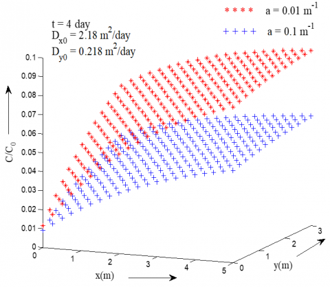
Figure 4. Dimensionless concentration distribution evaluated by analytical solution presented in Eq. (25) for two values of heterogeneous parameter in $0\,\,\le \,t\,<\,\,{{t}_{1}}\left( 5\,\text{day} \right)$
Figure 4 shows concentration distributions pattern predicted by the solution in Eq. (25) at two values of heterogeneous parameter $a=0.01$ and $0.1\,\text{(}{{\text{m}}^{\text{-1}}}\text{)}$. The calculations are conducted with the common values of parameters ${{D}_{{{x}_{0}}}}=2.18\,\text{(}{{\text{m}}^{\text{2}}}\text{/day)}$, ${{D}_{{{y}_{0}}}}=0.218\,\text{(}{{\text{m}}^{\text{2}}}\text{/day)}$ and $t=4.0\,\text{(day)}$. As expected, the concentration distribution became lower for higher heterogeneous parameter and higher for lower heterogeneous parameter. It may also observe that effect of heterogeneous parameter on the concentration distribution is relatively small near the inlet boundary.
Case-II: Figures (5-7) demonstrate the concentration distribution behaviour in the time domain ${{t}_{1}}\,\left( 5\,\text{day} \right)\,\le \,\,t\,\,<\,\,{{t}_{2}}\,\left( 10\,\text{day} \right)$ for the analytical solution obtained in Eq. (26).
Figure 5. Dimensionless concentration distribution evaluated by analytical solution presented in Eq. (26) at two different time for ${{t}_{1}}\,\left( 5\,\text{day} \right)\,\le \,\,t\,\,<\,\,{{t}_{2}}\,\left( 10\,\text{day} \right)$
Figure 5 illustrates the dimensionless concentration distribution for the point source along the longitudinal and lateral directions of the medium described by the solution in Eq. (26) computed for the common parameters, ${{D}_{{{x}_{0}}}}=2.18\,\text{(}{{\text{m}}^{\text{2}}}\text{/day)}$ , ${{D}_{{{y}_{0}}}}=0.218\,\text{(}{{\text{m}}^{\text{2}}}\text{/day)}$ and $a=0.01\,\text{(}{{\text{m}}^{\text{-1}}}\text{)}$ at $t\,=6$ and 9. It may be observed that concentration value is decrease with position and increases with time.
Figure 6. Dimensionless concentration distribution evaluated by analytical solution presented in Eq. (26) at two sets values of dispersion coefficient for ${{t}_{1}}\,\left( 5\,\text{day} \right)\,\le \,\,t\,\,<\,\,{{t}_{2}}\,\left( 10\,\text{day} \right)$
Figure 6 represents the effect of dispersion coefficient on dimensionless concentration distribution predicted by the present solution in Eq.(26) evaluated for two sets values of dispersion coefficients { ${{D}_{{{x}_{0}}}}=2.18\,\text{(}{{\text{m}}^{\text{2}}}\text{/day)}$ , ${{D}_{{{y}_{0}}}}=0.218\,\text{(}{{\text{m}}^{\text{2}}}\text{/day)}$ } and { ${{D}_{{{x}_{0}}}}=3.78\,\text{(}{{\text{m}}^{\text{2}}}\text{/day)}$ , ${{D}_{{{y}_{0}}}}=0.378\,\text{(}{{\text{m}}^{\text{2}}}\text{/day)}$ } at $t=9.0\,\text{(day)}$ and $a=0.01\,\text{(}{{\text{m}}^{\text{-1}}}\text{)}$ . It may be observed that distribution pattern of contaminant concentrations is nearly similar as in Figure (5). At particular position the concentration level is lower for lower dispersion coefficient and higher for higher dispersion coefficient.
Figure 7. Dimensionless concentration distribution evaluated by analytical solution presented in Eq. (26) for two values of heterogeneous parameter in ${{t}_{1}}\,\left( 5\,\text{day} \right)\,\le \,\,t\,\,<\,\,{{t}_{2}}\,\left( 10\,\text{day} \right)$
Figure 7 illustrates the solute transport from the point source along the longitudinal and lateral directions of the medium, described by the solution in Eq. (26) for two values of heterogeneous parameter $a\,=0.01$ , $\,0.1\text{(}{{\text{m}}^{\text{-1}}}\text{)}$ and other parameters values are taken as dispersion coefficient ${{D}_{{{x}_{0}}}}=2.18\,\text{(}{{\text{m}}^{\text{2}}}\text{/day)}$ , ${{D}_{{{y}_{0}}}}=0.218\,\text{(}{{\text{m}}^{\text{2}}}\text{/day)}$ and time $t=9\,\text{(day)}$ . It may be observed that the solute concentration decreases with position and heterogeneous parameter near and away from the source boundary. However, it starts decreasing with position until reaches a harmless level is achieved.
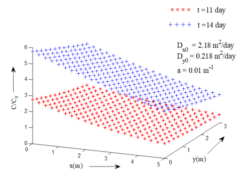
Figure 8. Dimensionless concentration distribution evaluated by analytical solution presented in Eq. (27) at two different time for $t\,\ge \,{{t}_{2}}\,\left( 10\,\text{day} \right)$
Case-III: Figures (8-10) demonstrate the concentration distribution behaviour in the time domain $t\,\ge \,{{t}_{2}}\,\left( 10\,\text{day} \right)$ for the analytical solution obtained in Eq. (27).
Figure 8 illustrates the same described by the solution in Eq.(27) at time $t=11$ and $14\text{(days)}$ with other input values ${{D}_{{{x}_{0}}}}=2.18\,\text{(}{{\text{m}}^{\text{2}}}\text{/day)}$ , ${{D}_{{{y}_{0}}}}=0.218\,\text{(}{{\text{m}}^{\text{2}}}\text{/day)}$ and $a=0.01\,\text{(}{{\text{m}}^{\text{-1}}}\text{)}$. It may be observed that the concentration level is much higher near inlet boundary and starts decreasing with position. The concentration pattern increases with time and decreases with position and after certain distance it becomes constant for all time.
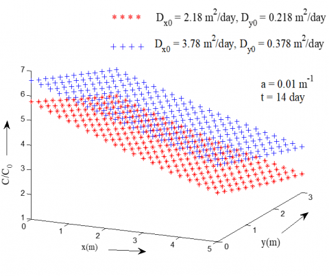
Figure 9. Dimensionless concentration distribution evaluated by analytical solution presented in Eq. (27) at two sets values of dispersion coefficient for $t\,\ge \,{{t}_{2}}\,\left( 10\,\text{day} \right)$
Figure 10. Dimensionless concentration distribution evaluated by analytical solution presented in Eq. (27) for two values of heterogeneous parameter for $t\,\ge \,{{t}_{2}}\,\left( 10\,\text{day} \right)$
Figure 9 demonstrates the effect of dispersion coefficient on the concentration profiles given by the solution in Eq. (27) for two sets values of dispersion coefficient as: { ${{D}_{{{x}_{0}}}}=2.18\,\text{(}{{\text{m}}^{\text{2}}}\text{/day)}$ , ${{D}_{{{y}_{0}}}}=0.218\,\text{(}{{\text{m}}^{\text{2}}}\text{/day)}$ } and { ${{D}_{{{x}_{0}}}}=3.78\,\text{(}{{\text{m}}^{\text{2}}}\text{/day)}$ , ${{D}_{{{y}_{0}}}}=0.378\,\text{(}{{\text{m}}^{\text{2}}}\text{/day)}$ } at $t=14\,\text{(day)}$ and $a=0.01\,\text{(}{{\text{m}}^{\text{-1}}}\text{)}$ . The effect of dispersion coefficient plays a significant role on distribution of solute. The pollutant attenuates continuously with position and time. It may be observed that the concentration level is lower for lower dispersion coefficient and higher for higher dispersion coefficient. The concentration pattern decreases with position until steady state is reached.
Figure (10) shows the distributions of the dimensionless concentration predicted by the solution given in Eq.(27) computed for two values of heterogeneous parameter as: $a\,=0.01$ and $\,0.1\,\text{(}{{\text{m}}^{\text{-1}}}\text{)}$ with common input values ${{D}_{{{x}_{0}}}}=2.18\,\text{(}{{\text{m}}^{\text{2}}}\text{/day)}$ , ${{D}_{{{y}_{0}}}}=0.218\,\text{(}{{\text{m}}^{\text{2}}}\text{/day)}$ and $t=14\,\text{(day)}$ . It may be observed that heterogeneity plays a significant role on concentration distribution. concentration attenuates with position and time. The concentration pattern decreases with heterogeneity parameter and position but after a certain distance it becomes constant for all time.
Analytical solutions are obtained for spatially dependent solute dispersion for varying input point source defined by Heaviside function in a two-dimensional semi-infinite porous medium with an appropriate realistic initial and boundary conditions. At the initial stage the aquifer domain is considered not solute free. Dispersion coefficient is considered proportional to square of groundwater velocity in both directions (longitudinal and lateral). The effects of various parameters are significantly observed on the concentration profiles. Laplace Integral Transformation Technique (LITT) is employed to get the analytical solutions. LITT is simpler, more viable and commonly used in assessing the stability of numerical solutions in more realistic dispersion problems. Two transformations have been used to obtain the analytical solutions. The effects of solute transport parameters on concentration profiles are evaluated in different time domains and demonstrated with help of graphs. The obtained analytical solutions may be helpful in predicting the concentration levels in the aquifer at any position and time and also useful for verifying the accuracy of numerical solutions.
|
$C$ |
Solute concentration, kg m-3 |
|
${{C}_{0}}$ |
Reference solute concentration, kg m-3 |
|
${{C}_{i}}$ |
Initial solute concentration, kg m-3 |
|
$u$ |
Longitudinal groundwater velocity, ms-1 |
|
$v$ |
Lateral groundwater velocity, ms-1 |
|
${{u}_{0}}$ |
Initial longitudinal groundwater velocity, ms-1 |
|
${{v}_{0}}$ |
Initial lateral groundwater velocity, ms-1 |
|
${{D}_{x}}$ |
Longitudinal dispersion coefficient, m2s-1 |
|
${{D}_{y}}$ |
Lateral dispersion coefficient, m2s-1 |
|
${{D}_{{{x}_{0}}}}$ |
Initial longitudinal dispersion coefficient, m2s-1 |
|
${{D}_{{{y}_{0}}}}$ |
Initial lateral dispersion coefficient, m2s-1 |
|
$x$ |
Longitudinal space variable, m |
|
$y$ |
Lateral space variable, m |
|
$X$ |
New longitudinal space variable, m |
|
$Y$ |
New lateral space variable, m |
|
$Z$ |
New space variable, m |
|
$a$ |
Heterogeneous parameter, m -1 |
|
$t$ |
Time variable, s |
|
${{t}_{1}}$ |
Beginning time of source activation, s |
|
${{t}_{2}}$ |
Ending time of source activation, s |
|
$s$ |
Laplace parameter |
|
${{c}_{1}}\,\And \,{{c}_{2}}$ |
Arbitrary constant |
|
$p,\,\,q\,\,\And \,r$ |
Parameter of time function |
|
$\bar{C}$ |
Laplace transform of ${C}$ |
|
$\left. \begin{align} & u(t-{{t}_{1}})\, \\ & u(t-{{t}_{2}}) \\\end{align} \right\}$ |
Heaviside function |
|
$\left. \begin{align} & {{D}_{0}},{{\gamma }_{0}},{{w}_{0}}\,, \\ & {{U}_{0}},\,{{U}_{1}},{{U}_{2}}, \\ & \,\alpha ,\,\beta ,\,\delta \\\end{align} \right\}$ |
New substituting constant |
[1] Gelhar, L.W. (1993). Stochastic Subsurface Hydrology. Prentice Hall. Englewood Cliffs. NJ.
[2] Freeze, R.A., Cherry, J.A. (1979). Groundwater. Prentice-Hall. New Jersey.
[3] Cirpka, O.A., Kitanidis, P.K. (2002). Numerical evaluation of solute dispersion and dilution in unsaturated heterogeneous media. Water Resour. Res., 38(11): 1220. https://doi.org /10.1029/2001WR001262
[4] Watson, K.K., Jones, M.J. (1982). Hydrodynamic dispersion during absorption in finite sand: the constant concentration case. Water Resources Research, 18(1): 91-100. https://doi.org/10.1016/S0309-1708(02)00022-2.
[5] Goode, D.J., Konikow, L.F. (1990). Apparent dispersion in transient groundwater flow. Water Resources Research, 26(10): 2339-2351. https://doi.org/10.1029/WR026i010p02339
[6] Watson, S.J., Barry, D.A., Schotting, R.J., Hassanizadeh, S.M. (2002). Validation of classical density-dependent solute transport theory for stable high-concentration-gradient brine displacements in coarse and medium sands. Advances in Water Resources, 25: 611-635. https://doi.org/10.1016/S0309-1708(02)00022-2
[7] Qiu, Y., Deng, B., Kim, C.N. (2011). Analytical solution for spatially dependent solute transport in streams with storage zone. J. of Hydrol. Eng., 16(8): 689-694. https://doi.org/10.1061/(asce)he.1943-5584.0000358
[8] Guerrero, J.S., Pérez Pimentel, L.C.G., Skaggs, T.H. (2013). Analytical solution for the advection-dispersion transport equation in layered media. Int. J. of Heat and Mass Transfer, 56: 274-282. https://doi.org/10.1016/j.ijheatmasstransfer.2012.09.011
[9] You, K., Zhan, H. (2013). New solutions for solute transport in a finite column with distance-dependent dispersivities and time-dependent solute sources. J. Hydrol., 487: 87-97. https://doi.org/10.1016/j.jhydrol.2013.02.027.
[10] Singh, M.K., Ahamad, S., Singh, V.P. (2014). One-dimensional uniform and time varying solute dispersion along transient groundwater flow in a semi-infinite aquifer. Acta Geophysica, 62(4): 872-892. https://doi.org/10.2478/s11600-014-0208-7
[11] Falta, R.W., Wang, W. (2017). A semi-analytical method for simulating matrix diffusion in numerical transport models. J. Contam. Hydrol., 197: 39-49. https://doi.org/10.1016/j.jconhyd.2016.12.00 7.
[12] Yadav, R.R., Kumar, L.K. (2018). Two-dimensional conservative solute transport with temporal and scale-dependent dispersion: Analytical solution. Int. J. of Advances in Mathematics, 2018(2): 90-111.
[13] Das, P., Akhter, A., Singh, M.K. (2018). Solute transport modelling with the variable temporally dependent boundary. Sadhana (Indian Academy of Sciences), 43(12): 1-11. https://doi.org/10.1007/s12046-017-0778-6.
[14] Yadav, R.R., Kumar, L.K. (2019). Solute transport for pulse type input point source along temporally and spatially dependent flow. Pollution, 5(1): 53-70. https://jpoll.ut.ac.ir/article_68933_1100d387f656c844306c6b7ede38fad3.pdf.
[15] Bear, J. (1972). Dynamics of fluid in porous media. Amri. Elsvier Publ. Co. New York.
[16] Van Genuchten, M. Th., Alves, W.J. (1982). Analytical solutions of the one-dimensional convective-dispersive solute transport equation. Technical Bulletin No.1661. US Department of Agriculture.
[17] Scheidegger, A.E. (1957). The physics of flow through porous media. Toronto. Canada: University of Toronto Press.
[18] Kumar, A., Jaiswal, D.K., Kumar, N. (2010). Analytical solutions to one-dimensional advection - diffusion equation with variable coefficients in semi-infinite media. J. of Hydrology, 380: 330-337. https://doi.org/10.1016/j.jhydrol.2009.11.008
[19] Carnahan, C.L., Remer, J.S. (1984). Non-equilibrium and equilibrium sorption with a linear sorption isotherm during mass transport through porous medium: Some analytical solutions. J. of Hydrology. 73: 227-258. https://doi.org/10.1016/0022-1694(84)90002-7
[20] Abramowitz, M., Stegun, I.A. (1970). Handbook of Mathematical Functions. First Edition. Dover Publications Inc. New York: 1019.
[21] Todd, D.K. (1980). Groundwater Hydrology; 2nd edn. John Wiley & Sons.