OPEN ACCESS
Final energy demand of residential sector accounts for about 25 % of the overall final consumption in the European region, mainly driven by space heating, space cooling, domestic hot water and cooking, which represent about 85 % of the total. Definition of effective policies towards decarbonisation of heat demand have been hindered so far by the lack of temporally- and spatially-detailed heat demand profiles, a key input for energy system optimisation models. This study tries to fill this gap by designing and validating a bottom-up thermodynamic lumped-parameters model for the Italian building stock. More specifically, the model grounds on a resistance-capacitance thermodynamic model, defined for: four building archetypes, five periods of construction and six building typologies corresponding to different climate zones. The model is applied to Italy and results classified based respectively on regional and hourly space and time resolutions. The model is validated based on temporally aggregated regional data. The model is used to assess the consequences of alternative building refurbishment/new construction scenarios towards Nearly Zero Energy Buildings (nZEBs), defined according to official Italian policy strategies: for each scenario, the change in heat demand and the change in share of appropriate domestic heating supply technologies are evaluated. Finally, sensitivity analysis is performed on the most critical parameters of the model.
residential building stock, heat demand, thermodynamic building model, energy modelling, nearly zero energy buildings
The integration of multiple energy sectors (power, heat, transport) into a multi-energy systems configuration is widely recognized as a pivotal prerequisite for fostering the penetration of renewable energy sources in the energy mix, in compliance with Paris Agreement decarbonization targets [1]. To this end, most profitable results and synergies can be experienced by acting on the residential heat demand [2]. The final energy demand of residential buildings accounts, in fact, for about 25 % of the overall final consumption in the European Union, primarily driven by heat loads: space heating, space cooling, domestic hot water and cooking represent up to 85 % of the total residential energy use in European Union (EU) [3]. Such energy uses present several opportunities for rapid and cost-effective sector-coupling and decarbonisation policies, such as the replacement of traditional heating technologies with highly-efficient heat pumps coupled with thermal storage [4] and the refurbishment of old buildings towards Nearly Zero Energy Buildings (nZEBs) [5].
Nonetheless, the residential heat sector presents several complexities and site-specific dynamics, which need to be carefully understood and assessed in order to design effective policies. The lack of clear, country-wide analyses demonstrating the synergies and benefits that may be ensured by heat-electricity integration and nZEBs diffusion at the Italian level has hindered so far the design of decarbonisation policies in this direction [6]. In fact, despite the increasing spatial and temporal resolution and the capability of integrating multiple energy sectors ensured by a new generation of open-source energy models (e.g. Calliope, Dispa-SET, oemof) [7], there is still a significant lack of corresponding detailed current and prospected residential heating and cooling demand profiles, required as a key input to such models. In most contexts, heating and cooling energy uses are not metered (preventing the use of experimental data), whilst models for their synthetic generation are hardly available at the required spatial scale and level of aggregation (i.e. regional or national) [8]. The most recent literature tries addressing this gap by designing country-wide bottom-up building stock models, allowing for a high degree of control and customisability (including simulation of future changes due to refurbishment), while also ensuring a good accuracy. For instance, Protopapadaki et al. [9] propose a Modelica-based implementation of a bottom-up model of the Belgian building stock, generating aggregate heating and cooling loads for different building archetypes with a high temporal resolution. Gendebien et al. [10] perform a similar analysis for the same context, but relying on lumped-parameters building archetypes for a more computationally-efficient aggregate simulation, accounting also for alternative refurbishment scenarios. Following a similar methodology, Patteeuw et al. [11] demonstrate how bottom-up models based on thermodynamic lumped-parameters building archetypes also entail the potential for a hard-linked integration with energy system models, enabling heating and cooling demand profiles to become an endogenous variable of the optimisation problem for demand-side management analyses. As a drawback, all the mentioned building stock models are highly context-specific and need to be adapted or entirely re-designed for each different countrywide policy study.
In this study, we design a bottom-up thermodynamic lumped-parameters model of the Italian residential building stock. The developed model ensures an easy adaptation to other contexts, while keeping a context-specific parametrization (with a NUTS-2 spatial level of aggregation). The mathematical model and its Python implementation are made available as open-source material, in line with the requirements of the open energy modelling philosophy, thus fostering their degree of transparency, reproducibility and adaptability [12]. Moreover, this work introduces the nZEB archetype for each Italian climatic zone, allowing to simulate alternative refurbishment scenarios and to evaluate how the penetration of such highly-efficient buildings might change regional heating and cooling demand profiles.
Section 2 provides a detailed discussion of how building archetypes are defined and aggregated, whilst the model validation and the results are provided in Section 3.
The methodological approach adopted for the bottom-up representation of the building stock is summarized in Figure 1. Archetypes are differentiated based on a) geometry, b) construction period, and c) climate-dependent construction materials (Figure 1).
Figure 1. Tree structure of archetype combinations
Four building geometries are defined to represent the variety of the Italian building stock, in accordance with ISTAT data [13], namely: single-family, double-family, multifamily and apartment block. In relationship with the evolution of the national legislation, also four construction periods (influencing materials and heat transfer coefficients) can be identified: before 1975; from 1976 to 1990; from 1991 to 2005; from 2006 to 2020. To these, a fifth construction period is added to characterise nZEBs, considering that, as prescribed by the Italian Law 90/2013, all private buildings to be constructed after December 31st 2020 will need to fall in such category. Finally, six climate-dependent groups of construction materials are considered, one for each Italian climatic area. This is made to account for the fact that, for instance, buildings of an identical type and period can be more or less insulated depending on the typical climate of their region. The combination of such options provides a total figure of 120 different building archetypes.
Sub-section 2.1 details how each building archetype is characterized by means of an independent thermodynamic lumped-parameters model. The thermophysical parameters required to populate each modelled archetype are derived from ISO standards and existing national or European projects, and they are discussed in sub-section 2.2. Sub-section 2.3 presents the methods adopted to characterise the nZEB archetypes based those constructed for the existing building stock. Sub-section 2.4 details how the large-scale aggregation of heating and cooling loads related to each building archetype is performed. Finally, sub-section 2.5 presents the defined nZEB penetration scenarios.
2.1 Lumped-parameters building modelling approach
Vivian et al. [14] discuss the suitability of various degrees of complexity of lumped-parameters (RC, resistance-capacitance) thermodynamic building models in reproducing the real trends of heating and cooling demand profiles. In particular, they demonstrate that, while both 5R1C and 7R2C models ensure a good degree of accuracy in reproducing peaks and seasonal trends of heat demand, the two-capacitance model ensures a significantly more accurate representation of cooling loads. Comparable benchmarks are suggested also by Georges et al. [15].
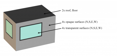
Figure 2. Schematic representation of a generic building archetype
Caldera et al. [16] have already proposed a lumped-parameter model for the representation of the Italian building stock, yet based on a single-capacitance approach. The approach for the calculation of the energy needs for heating and cooling adopted in the present study complies instead with the abovementioned findings and adopts a RC network model based on the ISO 52016:2017, further simplified by decreasing the number of temperature nodes in opaque elements. A whole building is indeed modelled as a single, box-shaped thermal zone (Figure 2) composed of 10 building elements (i.e. roof, floor, and four vertical walls – further differentiated into transparent and opaque surfaces). Each building element is characterized by a conductive resistance coupled with a capacitance applied to the node facing the internal volume (transparent building elements have null capacitance), by assuming that the mass is concentrated in a single node.
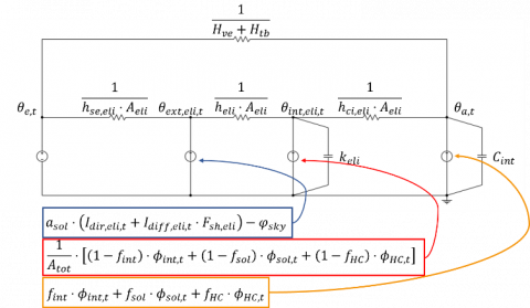
Figure 3 reports the equivalent-circuit representation, where it is assumed that there are no mechanical ventilation appliances, as they are not common in Italian existing residential buildings. The unknown variables are $θ_{int,eli,t}$, $θ_{ext,eli,t}$ and, alternatively, $Φ_{HC,t}$ or $θ_{a,t}$. It is worth noting that the scheme in Figure 3 represents, for simplicity, only one building element, coupled with the resistances representing the heat transfer coefficient for ventilation ($H_{ve}$) and thermal bridges ($H_{tb}$); an additional parallel connection between $θ_{e,t}$ and $θ_{a,t}$, with the same components reported in the figure, needs to be added for each additional building element.
Figure 3. Equivalent-circuit representation of the building thermodynamic model
Equations 1-4 show the corresponding mathematical model formulation, whereas the system is solved with respect to a fixed set-point temperature $θ_{a, t}$ for unknown $Φ_{HC,t}$. It is worth noting that the first two explicit equations resulting from the product (representing the energy balances on, respectively, the first and second node of the equivalent circuit from the left in Figure 3) are repeated for each of the 10 building elements, varying the parameters accordingly. The third equation resulting from the matrix-vector product, instead, represents the overall energy balance on the archetype.
$\mathbf{Ax}=\mathbf{b}$ (1)
$\mathbf{A}=\begin{bmatrix} h_{se,eli}+h_{eli} & -h_{eli} & 0\\ -h_{eli} & h_{eli}+h_{ci,eli}+\frac{k_{eli}}{△t} & -\frac{1-f_{HC}}{A_{tot}}\\ 0 & A_{eli}h{ci,eli} & f_{HC} \end{bmatrix} $ (2)
$\mathbf{x}=\begin{bmatrix} θ_{ext,eli,t} \\ θ_{int,eli,t}\\ Φ_{HC,t} \end{bmatrix}$ (3)
$\mathbf{b}=\begin{bmatrix} h_{se,eli}θ_{e,t}+a_{sol}(I_{dir,eli,t}F_{sh,eli}+I_{diff,eli,t}-φ_{sky} & \forall \in E\\ \frac{1}{A_{tot}}[(1-f_{int})Φ_{int,t}+(1-f_{sol})Φ_{sol,t}]+h_{ci,eli}θ_{a,t}+\frac{k_{eli}}{△t}θ_{int,eli,t-1} & \forall i \in E\\ \sum_i A_{eli}h_{ci,eli}θ_{a,t}+\frac{C_{int}}{△t}(θ_{a,t}-θ_{a,t-1})+(H_{ve}+H_{tb})(θ_{a,t}-θ_{e,t})-f_{int}Φ_{int,t}-f_{sol}Φ_{sol,t} & \end{bmatrix}$ (4)
2.2 Main thermophysical parameters and coefficients
Each building element is characterised by a number of thermophysical parameters that populate the system reported in Equation 1. The standard UNI/TR 11552:2014 provides the main thermophysical parameters of the opaque components that are most used in the Italian building stock. The standard also reports the most common wall, roof or floor stratigraphy with respect to the climatic zone and the period of construction of the considered building. Table 1 reports the calculated U-values for the example of single-family archetypes.
Table 1. U-values [W.m-2. K-1] for single-family buildings, by construction period, climatic zone and building element
|
Before 1975 |
A |
B |
C |
D |
E |
F |
|
Vertical Walls |
1.76 |
1.76 |
1.50 |
1.50 |
1.36 |
1.36 |
|
Roof |
1.74 |
1.74 |
1.74 |
1.74 |
1.74 |
1.74 |
|
Floor |
1.61 |
1.61 |
1.61 |
1.61 |
1.61 |
1.61 |
|
Transparent Elements |
5.00 |
5.00 |
4.60 |
4.60 |
4.60 |
4.60 |
|
1976-1990 |
A |
B |
C |
D |
E |
F |
|
Vertical Walls |
1.10 |
1.10 |
0.94 |
0.94 |
0.68 |
0.68 |
|
Roof |
1.46 |
1.46 |
1.46 |
1.46 |
0.98 |
0.98 |
|
Floor |
1.25 |
1.25 |
1.25 |
1.25 |
1.25 |
1.25 |
|
Transparent Elements |
5.00 |
5.00 |
3.20 |
3.20 |
3.20 |
3.20 |
|
1991 - 2005 |
A |
B |
C |
D |
E |
F |
|
Vertical Walls |
0.67 |
0.67 |
0.67 |
0.67 |
0.63 |
0.63 |
|
Roof |
1.10 |
1.10 |
1.10 |
1.10 |
0.74 |
0.74 |
|
Floor |
1.18 |
1.18 |
1.00 |
1.00 |
0.82 |
0.82 |
|
Transparent Elements |
5.00 |
5.00 |
3.20 |
3.20 |
3.20 |
3.20 |
|
2006-2020 |
A |
B |
C |
D |
E |
F |
|
Vertical Walls |
0.60 |
0.60 |
0.41 |
0.41 |
0.35 |
0.35 |
|
Roof |
0.38 |
0.38 |
0.35 |
0.35 |
0.31 |
0.31 |
|
Floor |
0.62 |
0.62 |
0.40 |
0.40 |
0.34 |
0.34 |
|
Transparent Elements |
4.00 |
4.00 |
2.60 |
2.60 |
2.20 |
2.20 |
Depending on the layers and materials adopted, a conductive heat transfer coefficient, $h_{eli}$, is evaluated for each element starting from the U value computed according to ISO 6946:2017, which specifies the characteristics related to the dynamic thermal behaviour of a complete building component and provides methods for their calculation. The calculation is reported in Equation 5.
$U=\frac{1}{h_{si,eli}+h_{eli}+h_{se}}$ (5)
where, $h_{si,el}$ and $h_{se,eli}$ are the internal and external surface heat transfer coefficients, comprising both convective and radiative heat transfer) are derived from ISO 13789:2017.
The same standard provides also values for the internal surface convective heat transfer coefficient, $h_{ci,eli}$, depending on the direction (vertical or horizontal) of the thermal flow on the i-th building element.
The overall heat exchange coefficient by (natural) ventilation ($H_{ve}$) is computed by means of Equation 6 as a function of the air flow rate $q_{V,t}$.
$H_{ve}=ρ_aC_aQ_{V,t}$ (6)
The calculation of the overall heat transfer coefficient for thermal bridges ($H_{tb}$) is reported in Equation 7.
$H_{tb}=\sum_kl_{tb,k}ψ_{tb,k}$ (7)
where, $l_{tb,k}$ and $ψ_{tb,k}$, respectively the length and the linear thermal transmittance of a linear thermal bridge, are gathered from 14683:2017. To this regard, an exception is represented by buildings realized after 2005; for this category, $H_{tb}$ is assumed equal to a 15 % increase of the overall heat transfer value due to transmission, as prescribed by “Decreto legislativo 19 agosto 2005, n.192”.
The remaining thermophysical coefficients are obtained from tabulated values contained in ISO 52016:2017, with the exception of the heat capacity of the building element ($k_{eli}$), which is considered applied on the internal node and is calculated according to ISO 13786:2005.
Special mention must be made of the shading reduction factor $F_{sh}$. The latter, representing the ratio between the actual and theoretical direct irradiance on a building element, can range between 0 and 1, i.e. from “null” to “complete” direct irradiance. Its assessment is highly building-specific, as it depends on detailed geometrical data on the building itself and on nearby obstacles, making it virtually impossible to compute a single average value for large-scale aggregates. For this work – based on a representative analysis carried out on a generic building in Turin, under the assumptions of a two-floors building with obstacles on four sides, as for a typical urban context – an average value of 0.75 is assumed. Nonetheless, possible deviations from this value are also identified in the range 0.50-1, and used to carry out a sensitivity analysis (sub-section 3.1).
2.3 nZEB archetype characterisation
The nZEB archetypes are characterised assuming they originate from a refurbishment intervention on existing buildings, as a result of the improvement of the insulation properties. In fact, the Italian “DM 26/06/2015” prescribes a set of minimum requirements that both new and refurbished buildings must satisfy to be considered nZEB. At the current stage of the work, aimed at defining the energy needs, the nZEB archetypes are defined considering the thermophysical performance of the envelope, neglecting the limits related to the energy appliances. The decree prescribes, for each climatic zone, a specific transmittance limit for each building element, without distinction between different building geometries (single-family, etc.). Accordingly, all transmittance values are assumed equal to the limit values prescribed for nZEBs (Table 2).
Table 2. U-values [W.m-2.K-1] limits for nZEBs, by climatic zone and building element
|
nZEB |
A |
B |
C |
D |
E |
F |
|
Vertical Walls |
0.43 |
0.43 |
0.34 |
0.29 |
0.26 |
0.24 |
|
Roof |
0.35 |
0.35 |
0.33 |
0.26 |
0.22 |
0.20 |
|
Floor |
0.44 |
0.44 |
0.38 |
0.29 |
0.26 |
0.24 |
|
Transparent Elements |
3.00 |
3.00 |
2.20 |
1.80 |
1.40 |
1.10 |
Achieving such limit values requires significant enhancements of the insulation properties of existing buildings. Required transmittance reductions for vertical walls range from -82.4 % to -16 %, depending on the building geometry and climatic zone, whilst reductions in the transmittance of transparent surfaces (windows) range from -78.3 % to -23.1 %. The envelope renovation must be carried out through processes of thermal insulation coating; a proper insulating material needs to be added to roof, ground floor and walls, while windows needs to be substituted. For vertical walls, fiberglass is considered the preferable insulating material, and the thickness of the additional insulation is calculated for each case as reported in Table 3.
Furthermore, the Italian “DM 26/06/2015” specifies that all U-value limits for nZEBs are intended as already comprehensive of all thermal bridges. Accordingly, the overall thermal bridges transmittance $H_{tb}$ is null for all nZEB archetypes.
Table 3. Thickness [cm] of fiberglass insulation to reach nZEB status, by climatic area and construction period
|
|
A |
B |
C |
D |
E |
F |
|
b.1975 |
6.7 |
6.7 |
8.6 |
10.6 |
11.8 |
13.0 |
|
1976-1990 |
5.4 |
5.4 |
7.1 |
9.1 |
9.0 |
10.2 |
|
1991-2005 |
3.2 |
3.2 |
5.5 |
7.4 |
8.5 |
9.8 |
|
2006-2020 |
2.5 |
2.5 |
1.8 |
3.7 |
3.8 |
5.0 |
2.4 Simulation algorithm and regional aggregation
The system of equations summarised by Equation 1 is implemented in a Python 3.6 environment and solved for each combination of geometry, period of construction and climate-dependent construction materials, with a province-scale resolution in terms of irradiance and external temperature data. The latter data are obtained from the database of the Comitato Termotecnico Italiano (CTI), which provides “typical-year” time series of climatic data for Italy based on the European Standard EN ISO 15927-4:2005.
The algorithm is also constrained to follow a set of rules aimed at reproducing real-life typical dynamics and Italian normative prescriptions. Firstly, a precise period in which heating is allowed is set for each climatic zone, in accordance with the Italian legislation (Table 4).
Table 4. Heating periods by climatic zone
|
Climatic zone |
Start Date |
End Date |
|
A |
December 1st |
March 15th |
|
B |
December 1st |
March 15th |
|
C |
November 15th |
March 31st |
|
D |
November 1st |
April 15th |
|
E |
October 15th |
April 15th |
|
F |
(No limitations) |
|
Secondly, each combination of archetype and district-scale temperature series is solved for three different possible thermostat regulation settings. These correspond to the most typical regulation settings of Italian households, as identified by Corrado et al. [17]. Table 5 reports the three possible settings for sunlight hours (07:00-22:00), where the high set point is assumed to be 20°C and the low set point 16°C. Night-hours regulation is instead assumed to be identical in all cases and corresponding to the low set point.
Table 5. Thermostat regulation settings for different user types
|
Setting |
Typical user |
Weekdays |
Weekends |
|
R1 |
Elderly People |
High set point all day |
High set point all day |
|
R2 |
Young couple with children |
Low set point from 09:00 to 16:00 |
High set point all day |
|
R3 |
Adult couple with teenagers |
Low set point from 09:00 to 18:00 |
High set point all day |
The logic by which the R1 setting is solved is here reported as an example: during the heating period, and if the outdoor temperature is lower than 18°C, the algorithm reformulates Equation 1 to compute $θ_{a, t}$ assuming the heating is initially off. Whereas $θ_{a, t}$ would fall below the pre-defined indoor comfort threshold – set at 20°C or 16°C depending on the period of the day – Equation 1 is solved in its standard form to compute the required $Φ_{HC,t}$ to keep comfort conditions.
In any other period, $Φ_{HC,t}$ is conversely set to provide, if outdoor temperature is above 25°C, cooling energy. An upper indoor comfort temperature threshold of 26°C is set for both day and night, and a similar resolution logic to that of the heating period is adopted to compute the cooling needs.
Finally, district-scale results are aggregated at regional (NUTS-2) level, based on the data by ISTAT [13] about the district and regional distributions of buildings associated with the defined archetypes (initially assuming a null penetration of nZEBs) and of households associated with the three defined patterns of thermostat control. In particular, the following shares (among all Italian households) are identified for each setting: 25.3 % for setting R1, 26.3 % for setting R2 and 48.4 % for setting R3.
2.5 Scenarios definition
Three scenarios of progressive building stock refurbishment policies towards nZEBs are considered. These are based on the expected penetration of nZEBs in Italy, in the short-to-medium term, according to three different sources, namely: the national strategies PANZEB and STREPIN (which set targets for 2020), and the European project ZEBRA2020 (which sets more ambitious targets for 2030). The rationale by which refurbishment policies are simulated is that older and more energy-intensive buildings (those constructed before 1975), which also represent the largest share of the current building stock, shall be renovated first. Accordingly, the nZEBs shares estimated by the three sources for the whole building stock are here applied following the abovementioned rationale. The resulting penetration of nZEBs is, in all cases, such that only buildings belonging to the oldest construction period are interested by the intervention. Table 6 summarises the scenarios and the corresponding percentage share of renovated buildings.
Table 6. Percentage share of renovated buildings in each scenario
|
|
Estimated Italian nZEB penetration (refurbishment) |
Corresponding refurbishment of buildings before 1975 |
|
BAU |
- |
- |
|
PANZEB |
1 % |
1.56 % |
|
STREPIN |
Single-family: 3.5 % Other geometries: 3 % |
Single-family: 5.39 % Other geometries: 4.80 % |
|
ZEBRA2020 |
35 % |
54.77 % |
3.1 Model validation and sensitivity
The validation of the model is performed on space heating data only, considering the lack of reliable references for regional or country-wide cooling loads. Even for space heating, the identification of reference values is complicated by the lack of reliable metered data. Accordingly, the proposed model is tested against both data gathered from Eurostat, based on a large-scale household questionnaire for the reference year 2017, and data estimated by the HotMaps project [18], based on a top-down statistical approach for the reference year 2012.
As reported in Table 7, the total space heating demand simulated by the proposed lumped-parameters model exceeds by 18.2 % the value estimated by Eurostat, which can be regarded as the most real-life relevant. This result is in line with the expectations for a series of simplifications assumed for such large-scale analysis, including: the designed building-stock model does not account for buildings contiguity both with other buildings and unconditioned thermal zones (that would slightly reduce the required heat load); the model assumes typical occupation patterns for all buildings and does not account for the fact that a certain share of residential buildings is probably not occupied for the entire year (due to vacations, etc.). Furthermore, whilst most of the values adopted in this study for the definition of the building stock rely on databases referred to the period 2010-2011, Eurostat questionnaire data are referred to the year 2017. It is therefore reasonable to assume that, within this period, non-negligible efficiency interventions on the Italian building stock might have occurred, reducing the total space heating demand. On the other hand, the model demonstrates its effectiveness in providing a significantly lower (-16.6 %) and finer estimate than those achievable by means of simplified, top-down statistical approaches, as the one adopted by HotMaps.
Table 7. Comparison of model results for space heating against reference values
|
|
Eurostat questionnaire |
HotMaps estimate |
Building-stock model |
|
Space heating (TWh/year) |
257.6 |
365.2 |
304.4 |
|
Diff % |
+18.2 % |
-16.6 % |
- |
The model results are also tested in relationship with the uncertainty associated with the assumed value, through a proper sensitivity analysis. Figure 4a shows, as a reference example, how such sensitivity has an almost negligible effect on the space heating load profile of a single-family house located in l’Aquila (one of the coldest districts); similarly, Figure 4b shows an only slightly more marked effect on the cooling load profile of a single-family house in Siracusa (one of the hottest districts). As reported in Table 8, analogous conclusions can be drawn as regards the yearly total demands. It can be concluded that the uncertainty associated with the determination of an average representative shading reduction factor has only limited implications on both hour-by-hour and yearly results, though further investigations on this topic might be valuable.
Table 8. Sensitivity analysis on
|
|
$F_{sh}=1.0$ |
$F_{sh}=0.75$ |
$F_{sh}=0.5$ |
|
Heating demand (TWh/year) |
299.2 |
304.4 |
309.6 |
|
Cooling demand* (TWh/year) |
51.7 |
45.8 |
40.0 |
|
*Theoretical maximum cooling demand assuming all buildings are equipped with air conditioning units |
|||
Figure 4. Sensitivity analysis on the shading reduction factor for: a) single-family heat load in l’Aquila, on January 22nd; and b) single-family cooling load in Siracusa, on July 20th
3.2 nZEB scenarios
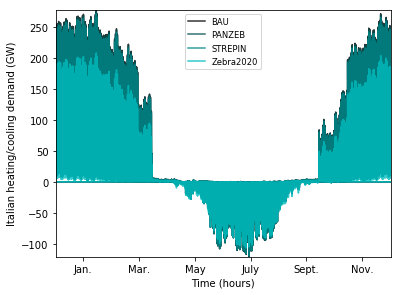
The marginal penetration of nZEBs assumed for 2020 by both PANZEB and STREPIN strategies demonstrate, as expected, only a minor impact on the national-aggregate heating demand, as shown in Figure 5 for a whole year. An even less significant impact is obtained for cooling loads (here represented as if all Italian residential buildings were equipped with air conditioning units). Such result highlights the need for pushing nZEB policies towards more ambitious targets in the upcoming years, as prospected, for instance, by the project ZEBRA2020. The results related to the latter scenario, in fact, demonstrate a much more valuable energy saving effect – still more marked for the heating demand, with a 35 % yearly reduction, as reported in Table 9.
Figure 5. Change in national-aggregate yearly heating and cooling loads for different nZEB penetration scenarios
Table 9. Summary of regional yearly heat demand [TWh] for different nZEB penetration scenarios
|
|
BAU |
nZEB1 |
nZEB2 |
nZEB3 |
|
Abruzzo |
7.7 |
7.7 |
7.5 |
5.1 |
|
Basilicata |
3.6 |
3.6 |
3.5 |
2.3 |
|
Calabria |
6.7 |
6.6 |
6.5 |
4.4 |
|
Campania |
16.1 |
15.9 |
15.6 |
10.8 |
|
Emilia-Romagna |
28.1 |
27.8 |
27.2 |
18.2 |
|
Friuli-VG |
9.5 |
9.4 |
9.2 |
6.1 |
|
Lazio |
18.0 |
17.9 |
17.5 |
11.7 |
|
Liguria |
5.7 |
5.6 |
5.5 |
3.9 |
|
Lombardia |
56.7 |
56.2 |
54.9 |
36.4 |
|
Marche |
8.9 |
8.8 |
8.6 |
6.0 |
|
Molise |
2.5 |
2.5 |
2.4 |
1.7 |
|
Piemonte |
36.7 |
36.4 |
35.6 |
24.3 |
|
Puglia |
14.9 |
14.8 |
14.5 |
10.2 |
|
Sardegna |
7.6 |
7.5 |
7.4 |
5.1 |
|
Sicilia |
13.3 |
13.1 |
12.9 |
8.9 |
|
Toscana |
18.7 |
18.5 |
18.1 |
12.6 |
|
Trentino-Alto Adige |
7.1 |
7.0 |
6.9 |
4.5 |
|
Umbria |
5.5 |
5.4 |
5.3 |
3.5 |
|
Valle D'Aosta |
1.2 |
1.2 |
1.2 |
0.8 |
|
Veneto |
35.8 |
35.4 |
34.6 |
22.7 |
|
ITALY |
304.4 |
301.4 |
294.7 |
199.2 |
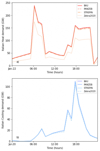
What is more, in the ZEBRA2020 scenario heating peak loads experience a significant reduction (around 30 %), as more clearly showcased by Figure 6.a. This result is particularly significant at the light of the increasing advocacy for heat-electricity integration policies. In fact, despite the benefits expected by such sector coupling measure, the transposition of current heat demand peaks into electricity loads would pose significant stress on the power-sector. Conversely, the generated results demonstrate that heat-electricity integration policies may have significantly lower drawbacks on the power sector, if implemented in parallel with a strong nZEB penetration.
Figure 6. Impact of nZEB penetration scenarios on: a) national-aggregate daily heating load, on January 22nd; and b) national-aggregate daily cooling load, for July 20th
Table 9 and 10 also provide valuable insights about the spatial distribution of heating and cooling demand, and about the corresponding achievable savings in each region. This may allow policy makers to identify those regions which showcase the highest relative energy-saving potential. In addition, the spatial detail ensured by the model further enhances its suitability for integration within high-resolution multi-layer energy modelling analyses, which are required to expand the findings of the present study towards broader technical and economic considerations.
Table 10. Summary of regional yearly (mamixum theoretical) cooling demand [TWh] for different nZEB penetration scenarios
|
|
BAU |
nZEB1 |
nZEB2 |
nZEB3 |
|
Abruzzo |
1.04 |
1.04 |
1.03 |
0.99 |
|
Basilicata |
0.40 |
0.40 |
0.39 |
0.38 |
|
Calabria |
1.99 |
1.98 |
1.97 |
1.78 |
|
Campania |
4.26 |
4.25 |
4.23 |
4.00 |
|
Emilia-Romagna |
2.97 |
2.97 |
2.97 |
2.95 |
|
Friuli-VG |
0.88 |
0.88 |
0.88 |
0.88 |
|
Lazio |
5.37 |
5.35 |
5.33 |
4.99 |
|
Liguria |
0.60 |
0.60 |
0.60 |
0.64 |
|
Lombardia |
5.83 |
5.83 |
5.84 |
5.96 |
|
Marche |
1.02 |
1.02 |
1.02 |
0.99 |
|
Molise |
0.10 |
0.10 |
0.10 |
0.11 |
|
Piemonte |
2.04 |
2.04 |
2.05 |
2.14 |
|
Puglia |
4.48 |
4.46 |
4.44 |
4.03 |
|
Sardegna |
1.38 |
1.38 |
1.37 |
1.31 |
|
Sicilia |
6.23 |
6.21 |
6.17 |
5.56 |
|
Toscana |
3.05 |
3.05 |
3.04 |
2.92 |
|
Trentino-Alto Adige |
0.25 |
0.25 |
0.25 |
0.27 |
|
Umbria |
0.78 |
0.78 |
0.77 |
0.73 |
|
Valle D'Aosta |
0.04 |
0.04 |
0.04 |
0.04 |
|
Veneto |
3.12 |
3.12 |
3.12 |
3.16 |
|
ITALY |
45.80 |
45.75 |
45.62 |
43.84 |
This study presented a novel bottom-up lumped-parameters thermodynamic model of the Italian residential building stock with NUTS-2 resolution, including also the possibility to simulate user-defined nZEBs refurbishment scenarios. The model, which generates residential heating and cooling demand profiles with a 1-hour temporal resolution in each region, is conceived for application within multi-layer energy modelling analyses.
The model demonstrates a good legitimacy and degree of accuracy, at the light of the simplifications introduced, compared to other available estimates of Italian yearly space-heating demand. Furthermore, the model showcases a satisfying robustness to potential uncertainties in the determination of regional-aggregate shading reduction factors.
The results related to the simulation of different nZEB penetration scenarios highlight that ambitious refurbishment policies are required to achieve significant results in terms of both total yearly heating and cooling demand savings and peak demand reductions. The penetration levels expected by 2020 only provide marginal benefits.
The hour-by-hour results achievable by the model are of particular interest in the framework of heat-electricity integration policies: in fact, the expected increase in electricity peak demand due to the transition towards electric heating may be positively counterbalanced by the reduction in final heating and cooling peak demand ensured by widespread nZEBs penetrations. Future work shall further explore these synergies by integrating the developed model within a multi-layer energy modelling framework.
[1] Mathiesen BV, Lund H, Connolly D, Wenzel H, Østergaard PA, Möller B, Nielsen S, Ridjan I, Karnøe P, Sperling K, Hvelplund FK. (2015). Smart energy systems for coherent 100 % renewable energy and transport solutions. Applied Energy 145: 139-154. https://doi.org/10.1016/j.apenergy.2015.01.075
[2] Bloess A, Schill WP, Zerrahn A. (2018). Power-to-heat for renewable energy integration: A review of technologies, modeling approaches, and flexibility potentials. Applied Energy 212: 1611–1626. https://doi.org/10.1016/j.apenergy.2017.12.073
[3] Eurostat. (2017). Energy consumption in households. [Online]. Available: https://ec.europa.eu/eurostat/statistics-explained/index.php/Energy_consumption_in_households. [Accessed: 02-Oct-2018].
[4] Lombardi F, Balderrama Subieta SL, Nicolo S, Pistolese S, Colombo E, Quoilin S. (2018). Modelling of a village-scale Multi-Energy System (MES) for the integrated supply of electric and thermal energy. 10th International Conference on System Simulation in Buildings 2018: 1-19.
[5] Belussi L, Barozzi B, Bellazzi A, Danza L, Devitofrancesco A, Fanciulli C, Ghellere M, Guazzi G, Meroni I, Salamone F, Scamoni F, Scrosati C. (2019). A review of performance of zero energy buildings and energy efficiency solutions. Journal of Building Engineering 25: 100772. https://doi.org/10.1016/j.jobe.2019.100772
[6] Lombardi F, Rocco MV, Colombo E. (2019). A multi-layer energy modelling methodology to assess the impact of heat-electricity integration strategies: The case of the residential cooking sector in Italy. Energy 170: 1249–1260. https://doi.org/10.1016/j.energy.2019.01.004
[7] Pfenninger S, Hirth L, Schlecht I, Schmid E, Wiese F, Brown T. (2018). Opening the black box of energy modelling: strategies and lessons learned. Energy Strategy Reviews 19: 63-71. https://doi.org/10.1016/j.esr.2017.12.002
[8] Clegg S, Mancarella P. (2018). Integrated electricity-heat-gas modelling and assessment, with applications to the Great Britain system. Part I: High-resolution spatial and temporal heat demand modelling. Energy, 1–11. https://doi.org/10.1016/j.energy.2018.02.079
[9] Protopapadaki C, Reynders G, Saelens D. (2014). Bottom-up modelling of the Belgian residential building stock: Impact of building stock descriptions. 9th International Conference on System Simulation in Buildings 1-10.
[10] Gendebien S, Georges E, Bertagnolio S, Lemort V. (2015). Methodology to characterize a residential building stock using a bottom-up approach: A case study applied to Belgium. International Journal of Sustainable Energy Planning & Management 4: 71–88. https://doi.org/10.5278/ijsepm.2014.4.7
[11] Patteeuw D, Bruninx K, Arteconi A, Delarue E, D’haeseleer W, Helsen L. (2015). Integrated modeling of active demand response with electric heating systems coupled to thermal energy storage systems. Applied Energy 151: 306-319. https://doi.org/10.1016/j.apenergy.2015.04.014
[12] Pfenninger S, Decarolis J, Hirth L, Quoilin S, Staffell I. (2016). The importance of open data and software: Is energy research lagging behind. Energy Policy 101: 211-215. https://doi.org/10.1016/j.enpol.2016.11.046
[13] ISTAT, ISTAT - Censimento Popolazione. 2011. [Online]. Available: http://dati-censimentopopolazione.istat.it/Index.aspx?DataSetCode=DICA_NUCLEI. [Accessed: 10-Oct-2018].
[14] Vivian J, Zarrella A, Emmi G, Carli MD. (2017). An evaluation of the suitability of lumped-capacitance models in calculating energy needs and thermal behaviour of buildings. Energy and Buildings 150: 447-465. https://doi.org/10.1016/j.enbuild.2017.06.021
[15] Georges E, Gendebien S, Bertagnolio S, Lemort V. (2013). Modeling and simulation of the domestic energy use in Belgium following a bottom-up approach. Clima Rehva World Congress & International Conference on Iaqvec. https://doi.org/10.1002/jpln.19600900129
[16] Caldera M, Puglisi G, Zanghirella F, Ungaro P, Cammarata G. (2018). Numerical modelling of the thermal energy demand in Italian households through statistical data. International Journal of Heat and Technology 36(2): 381–390. https://doi.org/10.18280/ijht.360201
[17] Corrado V, Ballarini I, Paduos S, Primo E, Madonna F. (2017). Application of dynamic numerical simulation to investigate the effects of occupant behaviour changes in retrofitted buildings. Proceedings of the 15th IBPSA Conference 2017, pp. 1862–1869. https://doi.org/10.26868/25222708.2017.499
[18] Mueller A, Fallahnejad M. (2019) HotMaps project - Heat density map. [Online]. https://gitlab.com/hotmaps/heat/heat_tot_curr_density.