OPEN ACCESS
Nonlinear hyperbolic heat conduction problems are analyzed thanks to the Cattaneo-Vernotte model, which takes what happens at very short times into account. First, the case of the coupled conductive-radiative heat transfer in planar and spherical media is considered. The accuracy of the Lattice Boltzmann heat conduction model coupled with an analytical layered spherical harmonics solution of the radiative transport equation is investigated. The effects of different parameters such as scattering albedo on both temperature and conductive heat flux distributions within the medium are studied for steady and transient states. The present predictions agree well with literature benchmarks. It is also shown that the parameters have a significant effect on both temperature profile and hyperbolic sharp wave front. Second, the non-Fourier heat conduction in a thermoelectric thin layer is investigated under several boundary conditions by performing a specific quadrupole method. The expressions of the temperature and the heat flux of the small-scale thermoelectric materials are obtained and the whole matrix formulation is given explicitly. Good agreement is observed between quadrupole temperature predictions and analytical results for the Fourier heat conduction problems.
analytical layered radiative solution, non-Fourier conduction, lattice Boltzmann method, quadrupole method, planar/spherical media, thermoelectricity
Simultaneously, transient conduction and/or radiation in participating media appears in many engineering systems and emerging technologies such as nanostructures, biological tissues, insulated foams, polymers, furnaces, heat pipes, combusting chambers and rocket propulsion, renewable energy applications using thermoelectric materials [1-3]. The amount and rate of heat, coupled to system properties and the surrounding govern the thermal response at both the microscopic and macroscopic scales. For transient heat flow during an extremely short period, the conduction process is well described by the hyperbolic heat conduction theory based on non-Fourier constitutive heat flux equations such as the Cattaneo – Vernotte heat flux equation, which implies a finite speed for the propagation of thermal perturbations [4-5]. In engineering practice, it is convenient to simulate the non-linear heat conduction behavior with commercial software such as ANSYS, FLUENT and TRNSYS [6-8]. However, it is interesting and suitable to develop semi analytical models for instance to make a thermodynamic analysis of a thermoelectric device [9], to estimate the maximum rate of heat pumping, to study the influence of one parameter, to use it for optimization or as an inverse model. Moreover, several modeling of the transient state is based on the convenient electrical analogy, Laplace transform and separation of the variables [10] finite difference/volume and the lattice Boltzmann (LBM) methods [11] to study thermoelectric self-cooling of devices. They are also convenient to solve the partial differential equation for a small time leg or for micro thermoelectric coolers [12].
At macroscopic scales, the time and spectral changes of radiative information are often considered as non-significant due to its very large propagation speed and gray medium assumption [13]. Hence, the radiation assessment involves an integro-differential radiative transfer equation (RTE) including three spatial and two angular variables. Furthermore, for present curvilinear shape, the differential form of the RTE coupled to the dependence of spatial/angular variables and the optically inhomogeneous complex media make the radiative transfer equation difficult to solve analytically except for some limiting cases [1, 2, 13]. Generally, the solutions of RTE found in the literatures are typically determined by numerical means and therefore, contain errors such as angular and spatial errors due to solution procedures. To mitigate the effects of error due to angular discretization, different approaches have been described in the literatures, including phase function renormalization, high order angular discretization, angular grid refinement [2, 11, 14-15]. However, the error due to spatial discretization depends to the considered approach around each grid node and to the selected method. In order to improve the accuracy of the solution, semi-analytical approach based on discrete ordinates has been developed recently by Ladeia et al. [16] for cylindrical media but limited to homogeneous and steady state transfer.
The present research is concerned: (1) firstly with the development of an analytical solution for radiation analysis in optically complex media of inhomogeneous graded index. The spherical harmonics method is then used for the development of an analytical radiative transfer solution. The non-linear hyperbolic heat conduction with temperature dependent thermal conductivity has been investigated through the lattice Boltzmann and finite volume methods; (2) and secondly with the complete one-dimensional transient hyperbolic heat transfer equation solved semi-analytically in order to obtain explicit expressions of the temperature and also of the heat flux in a thermoelectric layer. A quadrupole formulation of the hyperbolic partial differential equation taking the Thomson effect into account is then proposed for thin thermoelectric layer or medium considered at very short times.
2.1 Coupled conductive-radiative heat transfer in semi-transparent media
The local energy balance describes the transient conduction heat transfer in a medium:
$ρC_p ∂T/∂t=-∇(q_C+q_R )$ (1)
where ρ is the density, $C_p$ is the specific heat at constant pressure, $q_C$ is the conductive heat flux; T the temperature field at time t>0 and $q_R$ represents the radiative flux. The constitutive equation for conductive heat flux is stated by Cattaneo and Vernote through the expression [4-5]
$q_C (r,t+τ_cv )≈q_C (r,t)+τ_cv (T) (∂q_C)/∂t=-k_C (T)∇T$ (2)
The thermal conductivity of the material is considered in the form $k_C (T)=k_0 u(T)$ where $k_0$ represent the reference thermal conductivity. The temperature dependent time lag $τ_cv$ (T) is related to the constant speed $C_v$ by $τ_cv (T)=α(T)/C_v^2$. The boundary conditions of the thermal problem are known temperatures $T_0$ for left boundary, $T_L$ for right boundary, $T_∞$ is the initial temperature distribution. For combined mode of radiation and conduction, the radiative source is $∇q_R=κ_e (1-ω)[4n^2 σ_B T^4-2π∫_{-1}^{1 }I(r,μ)dμ]$ [2], where the parameter $κ_e$ is the extinction coefficient, $σ_B$ is the Stefan Boltzmann constant and ω is the single scattering albedo. The function $I(r,μ)$ is the radiative intensity known from RTE where the boundary conditions are [17, 18]
$I_1 (τ_0,μ)=b ̅(ϵ_0 I_b (T_0 )+2(1-ϵ_0 ) ∫_0^1I_1 (τ_0,-μ' ) μ' dμ' )+bI_1 (τ_0,-μ)$ (3a)
$I_(N_L ) (τ_L,μ)=ϵ_L I_b (T_L )+2(1-ϵ_L ) ∫_0^1I_{N_L} (τ_L,μ' ) μ' dμ'$ (3b)
where ϵ is the emissivity and b taking the value 1 for slab or hollow sphere and 0 for solid sphere ($b ̅=1-b$).
2.2 Non-Fourier conduction in thermoelements
Consider a single thermoelectric leg of length and cross-sectional area A. An electrical current I = JA enters uniformly into the element. As the thermoelectric material considered here is a thin thermoelectric layer, it is necessary to consider the hyperbolic law instead of the parabolic law of heat conduction [19]. The governing equation in a thin thermoelectric leg is the partial differential hyperbolic equation:
$ρC_p (∂T/∂t+τ_cv (∂^2 T)/(∂t^2 ))=∂/∂z (k_C ∂T/∂z)+J^2/σ-τJ ∂T/∂z$ (4)
The relevant properties are the electrical conductivity, the Thomson coefficient and finally is the relaxation time. To obtain the hyperbolic equation for a thermoelectric material, the steps are clearly detailed for instance in [20].
The first solution approach consists to solve the radiation transfer using the spherical harmonics in order to build the solution of Eq. (1) from Lattice Boltzmann method. Secondly, a specific quadrupole method is developed to solve the energy equation relative to a thin layer applied to thermoelectricity.
3.1 A layered radiative solution
The inhomogeneity and angular redistribution of radiative intensity increase the difficulties to build the analytical solution of the radiation equation. In order to construct a semi-analytical solution, the media is assumed to be a set of sub-layers with constant factor 1/τ. In such case, the radiative intensity in a single layer can be written as
$μ (∂I_k)/∂τ+(1-μ^2 ) a/τ (∂I_k)/∂μ+I_k-[1-ω] I_b (T)=ω/2 ∫_{-1}^1 Φ(μ'→μ) I_k (τ,μ' )dμ' $ (5)
where $ I_b=n^2 σ_B T^4/π$ is the blackbody intensity; $τ=κ_e r$ being the optical depth; $μ=cos(θ)$ is the polar direction cosine; and $Φ$ is the scattering phase function. For the constant a=0 and 1, the equation pertains to that for the slab and the spherical enclosure, respectively.
The radiative problem in each layer is solved using the spherical harmonics or PN method. Therefore, the radiative intensity is expanded as [2, 18]
$I_k (τ,μ)≈∑_{l=0}^NI_(l,k) (τ)P_l (μ)$ (6)
where $I_{l,k}$ are the radiative intensity moments to be determined and $P_l$ are the Legendre polynomials. Hence, applying recursive expression of $μP_l (μ)$ and combined to orthogonality condition of Legendre polynomials, the RTE is reduced to the matrix- vector form as
$A (dF^k)/dτ+(C+a/τ_k B) F^k=D^k;F^k=[I_{0,k},I_{1,k} ,⋯,I_{N,k}]^T$ (7)
and the component of matrices A,B and C are given, respectively, by
$A_{ll'}=1/(2l'+1) [l' δ_{l+1,l'}+(l'+1) δ_{l-1,l'}] $ (8a)
$B_{ll'}=(l' (l'+1))/(2l'+1) [δ_{l+1,l' }-(l'+1) δ_{l-1,l'}]$ (8b)
${{C}_{ll\text{ }\!\!'\!\!\text{ }}}={{\delta }_{ll\text{ }\!\!'\!\!\text{ }}}(1-\frac{(\omega {{a}_{l}})}{2l+1})$ (8c)
where δ is the Kronecker symbol; the components $D_l^k=δ_{0l}[1-ω(τ)] I_b (T)$ and $a_l$ is the scattering phase function coefficient. The Marshak boundary conditions are used in this study and written in matrix-vector form $A_0 F^1 (τ_0 )=D_0$ for inner and $A_L F^{N_L} (τ_L )=D_L$ for outer boundary [11, 18]
For transient heat transfer, the analytical solution of Eq. (7) for a single homogeneous and isothermal layer is similar to that developed by Ymeli and Kamdem [11] and Kamdem et al. [21] for planar media using double spherical harmonics method and discrete ordinates methods, respectively. The solution in each sub-layer is constructed by setting $F^k (τ)=R^k W^k (τ)$, where $R^k$ is the matrix of real eigenvector and $W^k (τ)$ is the vector of the characteristics intensity to be determined. Therefore, Eq. (7) is reduced to
$(dW^k)/dτ+Λ^k W^k=S^k=(AR^k )^{-1} D^k $ (9)
with $Λ^k$, the matrix of non-zero real eigenvalues λ of the system. Each decoupled component of characteristics radiative intensity $W^k$ can be solved analytically and independently as [21]
$W^k (τ)=exp[λ^k (τ_B^k-τ)] C^k+\widetilde{\exp }[λ^k (τ_B^k-τ)] S^k$ (10)
with $τ_B^k=τ_l^k+((1-k_a )(τ_r^k-τ_l^k))⁄2$, where $τ_l^k$ and $τ_r^k$ are the optical depth of the left and right interfaces of the $k^{th}$ layer. The constant $k_a$ is $|λ^k |⁄λ^k$ and the diagonal matrices exp and $\widetilde{\exp }$ are defined as
$exp\left( {{\lambda }^{k}}(\tau _{B}^{k}-\tau ))=diag({{e}^{\lambda _{0}^{k}(\tau _{B}^{k}-\tau )}},...,{{e}^{\lambda _{N}^{k}(\tau _{B}^{k}-\tau )}} \right)$ (11)
$\widetilde{\exp }[λ^k (τ_B^k-τ)]=(Λ^k )^(-1).(I-exp{λ^k (τ_B^k-τ)})$ (12)
where I is the identity matrix with the same size with exp. The determination of the constant $C^k$ from boundary conditions and continuity condition is reduced to the linear system MX=N [11] where components are given by
${{M}_{(i,j)}}\text{=}\left\{ \begin{matrix} \begin{matrix} {{A}_{0}}{{R}^{1}}exp[{{x}_{1}}(\tau )] & i=j=1 \\\end{matrix} \\ \begin{matrix} {{R}^{j}}exp[{{x}_{j}}(\tau )]{{\delta }_{(i-1,j)}}-{{R}^{(j+1)}}exp[{{x}_{(j+1)}}(\tau ]{{\delta }_{(i,j)}} & {} \\\end{matrix} \\ \begin{matrix} {{A}_{L}}{{R}^{({{N}_{L}})}}exp[{{x}_{({{N}_{L}})}}(\tau ) & i=j={{N}_{L}} \\\end{matrix} \\\end{matrix} \right.$ (13a)
${{N}_{i}}=\left\{ \begin{matrix} {{D}_{0}}-{{A}_{0}}{{R}^{1}}\widetilde{exp}[{{x}_{1}}(\tau )]{{S}^{1}}j=1 \\ {{R}^{(j+1)}}\widetilde{exp}[{{x}_{(j+1)}}(\tau )]{{S}^{(j+1)}}-{{R}^{j}}\tau [{{x}_{j}}(\tau )]{{S}^{j}} \\ {{D}_{L}}-{{A}_{L}}{{R}^{({{N}_{L}})}}\widetilde{exp}[{{x}_{({{N}_{L}})}}(\tau )]{{S}^{({{N}_{L}})}}j={{N}_{L}} \\\end{matrix} \right.$ (13b)
where $X=[C^1,C^2,…,C^{N_L}]^T$ is the vector containing the integration constant of all the layers, $N_L$ is the total number of sub-layers and $x_i (τ)=λ^i (τ_B^i-τ_i )$. The linear system is solved with LU factorization and the final solution in each layer is given by
$F^k (τ)=R^k exp[λ^k (τ_B^k-τ)] C^k+R^k\widetilde{\exp }[λ^k (τ_B^k-τ)] S^k $ (14)
The developed methodology presents the advantages that the volumetric radiation can be computed directly at a particular selected location with reasonable computational time allowing the coupled conduction and radiation heat transfer. The radiative flux $q_R$ is obtained from $q_R^k (τ)=4πI_(1,k) (τ)/3$.
In this study, the temperature is initially guessed using the distribution at the previous time step and the assumption of multilayers structure of the medium where temperature and are discretes and constants. This assumption has been also considered by Tan et al. [22] for radiation and Fourier’s conduction in graded index planar medium.
In addition, each layer has been splitting into nodes (including boundaries) to represent the solution given in Eq. (14). All these nodes are used to compute the solution of the conduction problem in the medium as a single layer.
3.2 Lattice Boltzmann method formulation (LBM)
The LBM is a computational method based on a mesoscopic description of heat flow, which better describes and captures sharp discontinuities of physical problems than the finite difference/volume methods [11, 23]. In order to simplify the energy equation with known radiative energy, we consider the dimensionless parameters as follows
$\eta =r/{{l}_{c}};\text{ }\xi ={{C}_{v}}t/{{l}_{c}},{{I}^{*}}=\frac{{{I}_{0}}(\eta )}{{{\sigma }_{B}}T_{h}^{4}/\pi },{{N}_{c}}=\frac{{{\kappa }_{e}}{{k}_{0}}}{4{{\kappa }_{B}}T_{h}^{3}}$ (15)
where $l_c=k_0⁄(ρC_p C_v )$ is the characteristic length of the problem, T_h is the reference temperature and N_c is the conductive-radiative parameter known also as Planck Number, the dimensionless time, distance, temperature $Θ=T/T_h$, and conductive heat flux $q_C^*=q_C/ρC_p T_h C_v$ are $ξ, η, Θ$, and $q_C^*$ respectively. Using this set of variables, Eqs. (1) and (2) are rewritten, as
$∂Θ/∂ξ+(∂q_c^*)/∂η=-a (q_C^*)/η-(κ_e l_c^2)/N_c ∇^* q_R$ (16a)
$∂q_C^*/∂ξ+∂Θ/∂η=-q_C^*/u(Θ)$ (16b)
with $∇^* q_R =κ_e [1-ω]{n^2 Θ^4-I^* }$ and $u(Θ)$ is a given function of temperature dependent thermal conductivity. The modified LBM equation due to radiation and non-Fourier is
$\frac{{{f}_{i}}}{\partial _{\xi }^{{}}}+{{\vec{e}}_{i}}.\nabla {{f}_{i}}=\frac{f{{_{i}^{e}}^{q}}-{{f}_{i}}}{{{\tau }_{M}}}-\frac{({{\kappa }_{e}}l_{c}^{2})}{2{{N}_{c}}}{{\nabla }^{*}}{{q}_{R}}-\frac{1}{2}\left( \frac{a}{\eta }/\hat{\eta }+\frac{{{e}_{i}}}{u(\theta )}) \right)q_{C}^{*}$ (17)
where $τ_M$ is the relaxation time, $f_i^{eq}$ is the equilibrium distribution function, $f_i$ is the particle distribution and $e ⃗_i$ is the moving velocity of the particles. For D1Q2 model, particles moves with two opposites unit velocities, $e_1 ⃗$ and $e_2 ⃗$. The relaxation time and vectors are $τ_M=u(Θ)+∆ξ/2$ [11, 23, 24]. After discretization, Eq. (17) is written as
${{f}_{i}}(\vec{\eta }+{{\vec{e}}_{i}}\Delta \xi ,\Delta +\Delta \xi )-{{f}_{i}}+\frac{\Delta \xi }{{{\tau }_{M}}}[f{{_{i}^{e}}^{q}}-{{f}_{i}}]+\frac{{{\kappa }_{e}}l_{c}^{2}}{2{{N}_{c}}}\Delta \xi {{\nabla }^{*}}{{q}_{R}}=\frac{\Delta \xi }{2}\left( \frac{a}{\eta }\hat{\eta }+\frac{{{{\vec{e}}}_{i}}}{u(\theta )} \right)q_{C}^{*}$ (18)
The temperature, conductive heat flux and equilibrium distributions are obtained from [11, 23, 24].
$Θ(η ⃗,ξ)=f_1 (η ⃗,ξ)+f_2 (η ⃗,ξ) $ (19a)
$q_C^* (η ⃗,ξ)=(e_1 ) ⃗.f_1 (η ⃗,ξ)+(e_2 ) ⃗.f_2 (η ⃗,ξ)$ (19b)
$f_i^{eq} (η ⃗,ξ)={Θ(η ⃗,ξ)+e ⃗_i.q_C^* (η ⃗,ξ)}/2$ (19c)
3.3 Quadrupole method
To solve the partial differential heat conduction equation, many different methods could be used but it is also very convenient to apply the Laplace transform, which transforms the partial differential equation into an ordinary differential equation in the Laplace domain. Let introduce p the Laplace variable and note To solve the partial differential heat conduction equation, many different methods could be used but it is also very convenient to apply the Laplace transform, which transforms the partial differential equation into an ordinary differential equation in the Laplace domain. Let introduce p the Laplace variable and note $L(f)=f ̅(p)=∫_0^{+∞}f(z,t)exp(-pt)dt$.
$(d^2 Θ ̅)/(dz^2 )-τJ/k_C (dΘ ̅)/dz-(ρC_p)/k_C p(1+pτ_cv ) Θ ̅(z,p)+J^2/(pσk_C )=0$ (20)
The roots of the characteristic associate equation are
${{\gamma }_{1,2}}=\frac{\tau J}{2{{k}_{C}}}\pm \sqrt{{{(\frac{\tau J}{2{{k}_{C}}})}^{2}}+\frac{\rho {{C}_{p}}}{{{k}_{C}}}p(1+p{{\tau }_{cv}})}$ (21)
As a consequence, the solution of the Eq. (20) is
$Θ ̅(z,p)=ξ_1 exp(γ_1 z)+ξ_2 exp(γ_2 z)+ϑ ̅(z)$ (22)
where $ϑ ̅(z)$ is a particular solution of Eq. (20) and $ξ_1, ξ_2$ are two constants depending on the boundary conditions. Two cases corresponding to different initial conditions are investigated to determine $ ϑ ̅(z)$:
IC0: the initial temperature within the leg is constant $T(z,t=0)=T_∞$ then it is obvious that
$\bar{\vartheta }(z)=\frac{{{J}^{2}}}{\rho {{C}_{p}}{{p}^{2}}\sigma (1+p{{\tau }_{c}}v)}+\frac{{{T}_{\infty }}}{p}$ (23)
IC1: the initial temperature is linear
$\bar{\vartheta }(z)=\frac{1}{p}(\frac{{{T}_{L}}-{{T}_{0}}}{L})z+\frac{\frac{{{J}^{2}}}{\sigma }+\frac{\tau J}{L}/({{T}_{L}}-{{T}_{0}})}{\rho {{C}_{p}}{{p}^{2}}(1+p{{\tau }_{c}}v)}+\frac{{{T}_{0}}}{p}$ (24)
Let for instance determine $ξ_1$ and $ξ_2$ in the most common case that is to say the thermoelectric thin layer is at the temperature $T_0$ and the side at $z=L$ is then at the temperature $T_L$. The equations corresponding to these boundary conditions are in the Laplace domain:
$Θ ̅(z=0,p)=0 ; Θ ̅(z=L,p)=(T_L-T_0 )/p$ (25)
Then $ξ_1$ and $ξ_2$ are determined as
${{\xi }_{1}}=\frac{\frac{{{J}^{2}}}{\rho {{C}_{p}}{{p}^{2}}\sigma (1+p{{\tau }_{c}}_{v})}(1-exp({{\gamma }_{2}}L)-\frac{({{T}_{L}}-{{T}_{0}})}{p})}{exp({{\gamma }_{2}}L)-{{\xi }_{2}}exp({{\gamma }_{1}}L)}$ (26a)
${{\xi }_{2}}=\frac{\frac{{{J}^{2}}}{\rho {{C}_{p}}{{p}^{2}}\sigma (1+p{{\tau }_{c}}_{v})}(exp({{\gamma }_{2}}L)-1+\frac{({{T}_{L}}-{{T}_{0}})}{p})}{exp({{\gamma }_{2}}L)-{{\xi }_{2}}exp({{\gamma }_{1}}L)}$ (26b)
Now, let express the heat flux which is a linear combination of the temperature and the derivative of the temperature (where $α_s$ is the Seebeck coefficient)
$φ=α_s IΘ-k_C A ∂Θ/∂z$ (27)
Considering Eqs (22) and (27), the Laplace transform of the heat flux is:
$\bar{\varphi }\left( z \right)=\left( {{\alpha }_{s}}I-{{k}_{C}}A{{\gamma }_{1}} \right)\text{ }{{\xi }_{1}}~exp\left( {{\gamma }_{1}}z \right)+\left( {{\alpha }_{s}}I-{{k}_{C}}A{{\gamma }_{2}} \right)\text{ }{{\xi }_{2}}\text{ }exp\left( {{\gamma }_{2}}z \right)+\overline{{{\varphi }_{2}}}\left( z \right)$ (28)
$\overline{{{\varphi }_{2}}}\left( z \right)\text{=}~\left( {{\alpha }_{s}}I.\bar{\vartheta }(z)-{{k}_{C}}A\frac{d\bar{\vartheta }(z)}{dz} \right)$ (29)
From a mathematical point of view, the quadrupole method belongs to the class of analytical unified exact explicit method for solving linear partial differential equations in simple geometries. H.S. Carlaw [25] first presented this approach for the conduction of heat in solids. The Laplace heat flux and temperature are analogue of the electrical current and electrical potential. To summarize, this method provides a transfer matrix for the medium that linearly links the input temperature–heat flux column vector at one side and the output vector at the other side. Let now determine the quadrupole corresponding to the case studied. Thanks to Eqs. (22) and (28)
$\text{ }\left[ \begin{matrix} \bar{\Theta }\left( {{z}_{i}} \right) \\ \bar{\varphi }\left( {{z}_{i}} \right) \\\end{matrix} \right]\text{=}{{M}_{p,i}}\left( \begin{matrix} {{\xi }_{1}} \\ \xi {}_{2} \\\end{matrix} \right)+{{U}_{p,i}}$ (30)
where
(31a)
$Mp.i=\left[ \begin{matrix} \bar{\vartheta }({{z}_{i}}) \\ {{a}_{s}}I\bar{\vartheta }({{z}_{i}})-{{k}_{c}}A\bar{\vartheta }({{z}_{i}})/dz \\\end{matrix} \right]$ (31b)
Considering the Eq. (26) at the both sides of the thermoelectric film, the quadrupole formulation of the problem is directly given by
$\text{ }\left[ \begin{matrix} \bar{\Theta }\left( 0 \right) \\ \bar{\varphi }\left( 0 \right) \\\end{matrix} \right]\text{=}{{M}_{p,0}}{{M}_{p,L}}^{-1}\left[ \begin{matrix} \bar{\Theta }\left( L \right) \\ \bar{\varphi }\left( L \right) \\\end{matrix} \right]-{{M}_{p,0}}{{M}_{p,L}}^{-1}{{U}_{p,L}}+{{U}_{p,0}}$ (32)
Thanks to this semi-analytical formulation, it is possible to plot the transient temperature along the thermoelectric film.
Toward the validation of the present development, the heat transfer occurring in three spatial configurations: the slab, the solid sphere and the hollow concentric spheres has been considered. For grid independent solution, the medium is divided into 90 layers for coupled PN – LBM, and each layer is split into ten grid points (including interfaces) to solve the radiation problem. For angular independent solution, a reasonable order P25 approximation has been found to be sufficient as recommended by Ymeli and Kamdem [18] for spherical geometry. The present section is organized as follows: the first part investigates the accuracy of the proposed methodology while the second part focus on the performances of the coupled PN–LBM in solving one-dimensional combined mode of radiative and non-Fourier conduction in inhomogeneous media. The third part investigates the effect of relaxation time on temperature field in thermoelement.
4.1 Steady state temperature distributions for inhomogeneous media
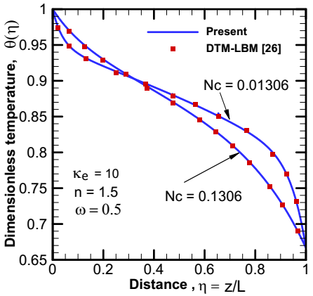
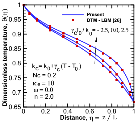
The PN – LBM code for computing the coupled volumetric radiation and heat conduction used in the present work was first benchmarked for steady state cases dealing with constant and temperature dependent thermal conductivity in 1-D planar medium. The temperature dependent thermal conductivity is considered in the form $k_c (T)=k_0+γ_C (T-T_0 )$. The left boundary has the emissivity $ϵ_0=0.2$ while the right boundary is considered as black and the optical thickness is taken to $κ_e L=10$ with scattering albedo $ω=0.0$.
Figure 1. Effect of conductive – radiative parameter on steady state temperature in a slab for $ϵ_0=0.2$ and $ϵ_L=1.0$
Figure 2. Effect of variable thermal conductivity on steady state temperature in a slab for $ϵ_0=0.2$ and $ϵ_L=1.0$
The temperature distributions with constant thermal conductivity are given in Figure 1 while the case with temperature dependent thermal conductivity is given in Figure 2. In order to establish the accuracy of the PN – LBM, these results are compared to those reported by Mishra et al. [26] based on Discrete Transfer Method (DTM). It is seen from these figures that the results of the present work match very well with those reported in the literatures.
The next considered problem is that of two concentric spheres where the inner radius has $R_0=0.5$ and outer radius $R_L=1.0$ with heated black boundaries $T_0=2T_L$. The extinction coefficient is $κ_e=2.0$ for isotropically scattering with constant thermal conductivity. The conduction-radiation parameter $N_C = 0.1 and 1.0$ with three scattering albedos $ω=0.1, 0.5 and 0.9$ are considered. The conductive heat flux $Q_C$ and total heat flux $Q_T$ at boundaries are presented in Table 2 for steady state and compared to Galerkin solutions [27] used as benchmark due to the high accuracy of the Galerkin method. Therefore, it can be observed in Table 2 that, the maximum relative errors for $Q_C (R_0 )$, $Q_C (R_L )$, $Q_T (R_0 )$ and $Q_T (R_L )$ are 0.3854 %, 0.5154 %, 0.4674 %, and 0.6146 % respectively. So, the developed methodology for coupled heat transfer shows good agreement with benchmark solutions for all the cases presented.
Table 1. Dimensionless conductive and total heat flux at the inner/outer black sphere with $κ_e R_L=2.0$, and $T_0=2T_L$ with $Q_C=R_L q_C/k_0 T_0$ and $Q_T=R_L (q_C+q_R )/k_0 T_0$
|
|
Conductive heat fluxes |
||||
|
Present |
Galerkin [27] |
||||
|
$N_c$ |
$ω$ |
$Q_C (R_0)$ |
$Q_C (R_L)$ |
$Q_C (R_0)$ |
$Q_C (R_L)$ |
|
0.1 |
0.1 |
2.5069 |
0.7066 |
2.5166 |
0.7100 |
|
0.5 |
2.3156 |
0.6413 |
2.3233 |
0.6426 |
|
|
0.9 |
2.0705 |
0.5372 |
2.0728 |
0.5378 |
|
|
1.0 |
0.1 |
2.0577 |
0.5211 |
2.0560 |
0.5238 |
|
0.5 |
2.0335 |
0.5143 |
2.0339 |
0.5156 |
|
|
0.9 |
2.0125 |
0.5040 |
2.0073 |
0.5049 |
|
|
|
Total heat fluxes |
||||
|
$Q_T (R_0)$ |
$Q_T (R_L)$ |
$Q_T (R_0)$ |
$Q_T (R_L)$ |
||
|
0.1 |
0.1 |
6.0774 |
1.5090 |
6.0519 |
1.5130 |
|
0.5 |
5.9487 |
1.4818 |
5.9433 |
1.4858 |
|
|
0.9 |
5.8241 |
1.4526 |
5.7970 |
1.4493 |
|
|
1.0 |
0.1 |
2.4002 |
0.5983 |
2.4080 |
0.6020 |
|
0.5 |
2.4034 |
0.5962 |
2.3954 |
0.5988 |
|
|
0.9 |
2.3896 |
0.5937 |
2.3797 |
0.5949 |
|
4.2 Transient temperature for nonhomogeneous media
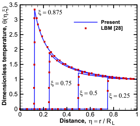
One of the particular cases of combined conduction-radiation problems correspond to the purely scattering medium with $ω=1.0$ where conduction equation (Eq.3) and radiative heat transfer equation (Eq.4) are decoupled and evolve separately. The considered problem concerns the solid sphere with constant thermal conductivity and throughout this study, the constant thermal speed is taken in such that $C_v R_L/2α_0=1.0$, with $R_L=1.0$. By selecting four time levels $ξ=C_v t/(R_L-R_0 ) = 0.25, 0.5, 0.75 and 0.875$, the corresponding transient temperature distributions are given in Figure 3 and compared to those of Mishra and Sahai [28] based on LBM. It should be note that, the benchmark solutions are considered as exact solutions due to the ability of the LBM to accommodate the thermal wave front. The most visible observation to be drawn is that temperatures increase or decrease suddenly. This behavior indicates the presence of the thermal wave front moving from the surface towards the center. The present Figure shows that, the LBM solution build in this work produces the same results with the implemented LBM in the literatures.
Figure 3. Temperature distributions at four time steps $ξ=0.25$, $ξ=0.5$, $ξ=0.75$ and $ξ=0.875$ for solid sphere
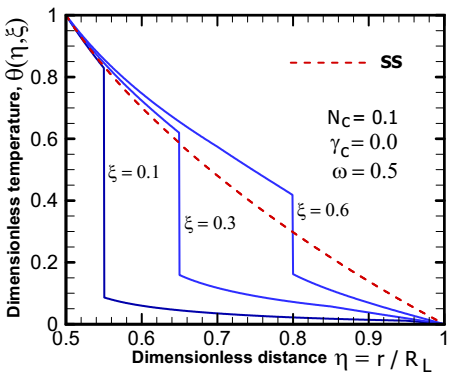
Figure 4. Temperature distributions at four-time steps $ξ=0.1$, $ξ=0.3$, $ξ=0.6$ and $ξ=6.2$ for $γ_C=0.0$
For the next considered case, the medium absorb 50% of radiation energy ($ω=0.5$) with $κ_e=1.0$, $R_0/R_L =0.5$ and conduction-radiation parameter $N_c=0.1$. The temperature distributions for hollow concentric spheres at four-time levels including the steady state (SS) $ξ=0.1$, $ξ=0.3$, $ξ=0.6$ and $ξ=6.2$ are presented in Figure 4. The thermal wave front moves from inner hot boundary to outer cold boundary and the temperature of the unperturbed zone increase with time, which is the contribution of thermal radiations.
4.3 Effect of variable thermal conductivity on transient temperature
Considering the solid sphere heated at the surface, the effect of temperature dependent thermal conductivity $k_c (T)=k_0 [1+β_C T]$ is now investigated with three values of $γ_C=β_C T_h$ for both conduction and radiation phenomena. The conduction-radiation number is taken to be $N_c=0.1$ and $ω=0.5$. Figure 5 depicts the temperature field for $γ_C = -0.5, 0.0 and +0.5$ at time levels $ξ=0.3$ and $ξ=0.6$. It is seen from this figure that, the increase of $γ_C$ parameter improves the temperature profile in the media and negative values of $γ_C$ strongly affect the temperature field than positive values. This may be attributed to the fact that for positive $γ_C$, the thermal conductivity increases and therefore improves the thermal transfer by conduction.
Figure 5. Effect of variable thermal conductivity on temperature field for $ω=0.5$, $Nc=0.1$ and $κ_e=1.0$ in solid sphere $(a) ξ=0.1$ $(b) ξ=0.3$ and $(c) ξ=0.6$
4.4 Effect of relaxation time on transient temperature for thermoelement
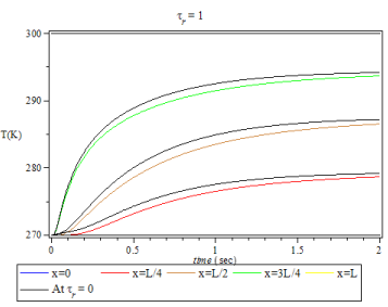
Thanks to semi-analytical method based on Laplace transform and quadrupole matrix formulation, the effect of thermal relaxation time on the transient temperature along the thermoelectric film is now investigated. The time variation of temperature at different coordinates $z=0$, $z=L/4$, $z=L/2$, $z=3L/4$ and $z=L$ is plotted in Figure 6. Four values of relaxation times are considered $τ_cv = 0.1s, 1s, 10s and 100s$ with the boundary conditions $IC0: T_∞=T_0=270K$ and $T_L=300K$. It is seen in this figure that for small relaxation times, there is not notably difference between the Fourier and non-Fourier states. As relaxation time increases, temperatures obtained with Fourier law are greater than those produce with non-Fourier law of thin layer
(a) Relaxation time $τ_cv$= 0.1s
(b) Relaxation time $τ_cv$= 1s
(c) Relaxation time $τ_cv$= 10s
Figure 6. Effect of relaxation time on temperature field of thermoelectric thin layer
The transient coupled non-Fourier conduction with radiation heat transfer in an inhomogeneous, scattering and gray medium with graded index is investigated. The analytical layered solution of radiation is developed based on linear algebra approach in complex media while the lattice Boltzmann method is used to solve the non-linear hyperbolic energy equation and compared with benchmark solutions. The contribution of radiation on the transient temperature distributions in the medium was graphically examined using three radiation parameters: temperature dependent thermal conductivity, single scattering albedo and conduction-radiation parameter. The obtained results show good agreement with benchmark solutions of radiative heat flux, steady state and transient temperature distributions. It was found that the radiation effect is more pronounced for high value of refractive index or low values of the single scattering albedo; conduction-radiation parameter while this contribution is less effective for anisotropic scattering coefficient. Through these calculations, it was found that although the hyperbolic sharp wave front of non-Fourier conduction becomes smoother when strong radiative heat transfer is taken into account, it can be damped or emphasized with the effect of thermal conductivity and the scattering albedo. The present study demonstrates that the proposed analytical layered solution for radiation coupled to Lattice Boltzmann method for non-linear hyperbolic conduction is accurate and suitable for combined radiation-conduction problems in complex media. In the case of thermoelectric elements, the development of a specific quadrupole applied to thermoelectricity allows to obtain the transient behavior of a film under several boundary conditions, to take into account what happens at very short times and to investigate the effect of relaxation times on the thermogram.
a=constant taken 0 for slab and for 1 sphere
A,B,C=matrices for angular discretized RTE
Cv=speed of the thermal wave (m.s-1)
Cp=specific heat at constant pressure (J.kg-1. K-1)
D=source vector for radiative transfer equation
$e ⃗$=velocities of the particle distribution functions
f=particle distribution function
F=vector of intensity moment
I=radiative intensity (W.m-2.Sr-1)
J=current density
kc=thermal conductivity (W.m-1.K-1)
L=length of the geometry (m)
Nc=conduction-radiation parameter
NL=total number of layers of the medium
Pl=Legendre polynomial
q=heat flux (W.m-2)
r,z=spatial variable (m)
R=matrix of eigenvectors
s=source term of the ordinary differential equation
T=temperature distribution (K)
t=time variable (s)
u=temperature dependent function
W=vector of radiative intensity moment
Greek symbols
α=thermal diffusivity (m2.s-1)
γ=dimensionless coefficient of thermal conductivity
δ=Kronecker symbol
ϵ=emissivity
η dimensionless distance
Θ dimensionless temperature
Λ matrix of real eigenvalue
λ eigenvalue
ξ dimensionless time or constant in thermoelectricity
ρ material density (kg.m-3)
σ Stefan-Boltzmann constant (5.67 × 10⁻⁸ W. m−2.K−4)
$κ_e$=extinction coefficient (m-1)
τ=optical depth
$τ_B$=optical thickness of a given layer
$τ_c$ relaxation time in non-Fourier conduction (s)
$τ_M$ thermal relaxation time for LBM model
Φ scattering phase function
ω scattering albedo
Superscripts
eq=equilibrium state
k=order of the given layer
T=transpose vector
Subscripts
c=conductive
h=reference
R=radiative
[1] Lazard M, Andre S, Maillet D, Baillis D, Degiovanni A. (2001). Flash experiment on a semitransparent material: Interest of a reduced model. Inverse Problems in Engineering 9(4): 413-429. http://doi.org/10.1080/174159701088027772
[2] Howell JR, Mengüç MP, Siegel R. (2015). Thermal Radiation Heat Transfer 6th ed. Taylor and Francis, CRC Press: New York. http://doi.org/10.1115/1.3607834
[3] Zheng XF, Liu CX, Yan YY, Wang Q. (2014). A review of thermoelectrics research – Recent developments and potentials for sustainable and renewable energy applications. Renewable and Sustainable Energy Reviews 32: 486-503. http://doi.org/10.1016/j.rser.2013.12.053
[4] Özişik MN, Tzou DY. (1994). On the wave theory in heat conduction. Journal of Heat Transfer 116(3): 526-535. http://doi.org/10.1115/1.2910903
[5] Zhou J, Zhang Y, Chen JK. (2008). Non-Fourier heat conduction effect on laser-induced thermal damage in biological tissues. Numerical Heat Transfer Part A 54: 1–19. http://doi.org/10.1080/10407780802025911
[6] Chen WH, Wang CC, Hung CI, Yang CC, Juang RC. (2014). Modeling and simulation for the design of thermal-concentrated solar thermoelectric generator. Energy 64(1): 287-297. http://doi.org/10.1016/j.energy.2013.10.073
[7] Espinosa N, Lazard M, Aixala L, Scherrer H. (2010). Modeling thermoelectric generator applied to diesel automotive heat recovery. Journal of Electronic Materials 39(9): 1446-1455. http://doi.org/10.1007/s11664-010-1305-2
[8] Massaguer E, Massaguer A, Montoro L, Gonzalez JR. (2014). Development and validation of a new TRNSYS type for the simulation of thermoelectric generators. Applied Energy 134: 65-74. http://doi.org/10.1016/j.apenergy.2014.08.010
[9] Chen J, Yan Z, Wu L. (1997). Nonequilibrium thermodynamic analysis of a thermoelectric device. Energy 22(10): 979-985. http://doi.org/10.1016/S0360-5442(97)00026-1
[10] Martínez A, Astrain D, Rodríguez A. (2011). Experimental and analytical study on thermoelectric self-cooling of devices. Energy 36(8): 5250-5260. http://doi.org/10.1016/j.energy.2011.06.029
[11] Ymeli LG, Kamdem THT. (2017). Hyperbolic conduction-radiation in participating and inhomogeneous slab with double spherical harmonics and lattice Boltzmann methods. ASME Journal of Heat Transfer 139(4): 1-14.
[12] Lazard M, Goupil C, Fraisse G, Scherrer H. (2012). Thermoelectric quadrupole of a leg to model transient state. Journal of Power and Energy Proc. IMechE 226: 277-282, https://doi.org/10.1177/0957650911433240
[13] Zhao JM, Liu LH. (2017). Radiative transfer equation and solutions. In: Kulacki F. (eds) Handbook of Thermal Science and Engineering. http://doi.org/10.1007/978-3-319-32003-8_56-1
[14] Hunter B, Guo Z. (2015). Applicability of phase – function normalization techniques for radiation transfer computation. Numerical Heat Transfer 67: 1-24. http://doi.org/10.1080/10407790.2014.949516
[15] Ge WJ, Michael F, Modest MF, Roy, S. (2016). Development of high-order PN models for radiative heat transfer in special geometries and boundary conditions. Journal of Quantitative Spectroscopy & Radiative Transfer 172: 98–109. http://doi.org/10.1016/j.jqsrt.2015.09.001
[16] Ladeia C, Bardo Bodmann EJ. Vilhena MT. (2018). The radiative conductive transfer equation in cylinder geometry: Semi-analytical solution and a point analysis of convergence. Journal of Quantitative Spectroscopy & Radiative Transfer 217: 338–352.
[17] Tsai JR, Ozisik MN. (1989). Radiations spherical symmetry with anisotropic scattering and variable properties. Journal of Quantitative Spectroscopy and Radiative Transfer 42(3): 187–199. http://doi.org/10.1016/j.jqsrt.2018.06.012
[18] Ymeli LG, Kamdem THT. (2015). High-order spherical harmonics method for radiative transfer in spherically symmetric problems. Computational Thermal Sciences 7(4): 353-371. http://doi.org/10.1615/ComputThermalScien.2015014843
[19] Lazard M, Goupil C, Fraisse G, Scherrer H. (2012). Thermoelectric quadrupole of a leg to model transient state. Journal of Power and Energy, Proc. IMechE 226: 277-282. https://doi.org/10.1177/0957650911433240
[20] Alata M, Al-Nimr MA, Naji M. (2003). Transient behavior of a thermoelectric device under the hyperbolic heat conduction model. International Journal of Thermophysics 24(6): 1753-1768. http://doi.org/10.1023/b:ijot.0000004103.26293.0c
[21] Kamdem THT, Ymeli LG, Tapimo R. (2017). The discrete ordinates characteristics solution to the one-dimensional radiative transfer equation. Journal of Computational and Theoretical Transport 46(5): 346-365. http://doi.org/10.1080/23324309.2017.1352519
[22] Tan H, Yi H, Luo J, Dong S. (2005). Effects of graded refractive index on steady and transient heat transfer inside a scattering semitransparent slab. Journal of Quantitative Spectroscopy and Radiative Transfer 96(3-4): 363–381. http://doi.org/10.1016/j.jqsrt.2004.12.034
[23] Mishra SC, Sahai H. (2012). Analyses of non-Fourier heat conduction in 1-D cylindrical and spherical geometry –An application of the lattice Boltzmann method. International Journal of Heat and Mass Transfer 55: 7015-7023. http://doi.org/10.1016/j.ijheatmasstransfer.2012.07.014
[24] Varmazyar1 M, Bazargan M. (59). Development of a thermal lattice Boltzmann method to simulate heat transfer problems with variable thermal conductivity. International Journal of Heat and Mass Transfer 59: 363-371. http://doi.org/10.1016/j.ijheatmasstransfer.2012.12.014
[25] Carslaw HS. (1922). Introduction to the mathematical theory of heat in solids. Monatshefte für Mathematik und Physik 32(1): A27-A28. http://doi.org/10.1007/BF01696928
[26] Mishra SC, Krishna NA, Gupta N, Chaitanya GR. (2008). Combined conduction and radiation heat transfer with variable thermal conductivity and variable refractive index. International Journal of Heat and Mass Transfer 51(1-2): 83-90. http://doi.org/10.1016/j.ijheatmasstransfer.2007.04.018
[27] Jia G, Yener Y, Cipolla J. (1991). Radiation between two concentric spheres separated by a participating medium. Journal of Quantitative Spectroscopy and Radiative Transfer 46(1): 11-19. http://doi.org/10.1016/0022-4073(91)90062-u
[28] Mishra SC, Sahai H. (2012). Analyses of non-Fourier heat conduction in 1-D cylindrical and spherical geometry – An application of the lattice Boltzmann method. International Journal of Heat and Mass Transfer 55: 7015-7023. http://doi.org/10.1016/j.ijheatmasstransfer.2012.07.014