Erroumayssae Sabani![]() | El Mehdi Loualid
| El Mehdi Loualid![]() | Hicham El Hadraoui
| Hicham El Hadraoui![]() | Kossai Fakir
| Kossai Fakir![]() | El Mehdi Laadissi
| El Mehdi Laadissi![]() | Adil Balhamri | Chouaib Ennawaoui*
| Adil Balhamri | Chouaib Ennawaoui*![]() | Azzeddine Azim
| Azzeddine Azim
© 2024 The authors. This article is published by IIETA and is licensed under the CC BY 4.0 license (http://creativecommons.org/licenses/by/4.0/).
OPEN ACCESS
Artificial Intelligence (AI) plays a crucial role in defect prediction within the context of Industry 4.0. By leveraging advanced machine learning algorithms, AI analyzes vast amounts of data from industrial processes to detect patterns indicative of potential faults. This predictive capability not only enhances maintenance efficiency but also minimizes downtime by enabling proactive interventions. In this paper, the authors evaluated the performance of three distinct training functions for ANNs used to diagnose bearing faults in a turbogenerator set: Levenberg-Marquardt, Bayesian Regularization, and Scaled Conjugate Gradient. The turbogenerator generated the dataset for this study, which was made up of a variety of input and output parameters. Based on the correlation coefficient (R) between the predicted and actual target values, each training function's performance was assessed. The results we achieved show that the output parameters of the turbogenerator set could be correctly predicted by all three training functions. However, the Bayesian Regularization algorithm had the lowest mean squared error (MSE) at epoch 1000, indicating that it had the best overall performance. The results produced indicated how each training function performed over time. According to these results, the Bayesian Regularization approach might be the best choice for forecasting the turbogenerator sets' output characteristics during bearing defect diagnostics. The results of this work show that choosing an adequate training function for ANN models is crucial for maximizing the accuracy of turbogenerator set predictions, notably in the diagnosis of bearing faults. Researchers and professionals in the field of diagnosing bearings faults and turbogenerator set problems may find these studies helpful.
ANN, Levenberg-Marquardt, Bayesian regularization, scaled conjugate gradient, MSE
Numerous industries, including manufacturing, power generation, transportation, and aerospace, depend heavily on rotating machinery. The most frequent parts used in rotating machinery are bearings, which support the shafts and guarantee a steady rotation. However, there are numerous faults that can affect bearings, including wear, cracks, defects, and lubrication problems. These faults can result in performance loss, downtime, and even catastrophic failures.
For rotating machinery to be reliable, safe, and efficient, bearing defects must be identified and treated as soon as possible. Numerous methods, including vibration analysis, acoustic emission monitoring, temperature measurement, and oil analysis, have been developed over time for diagnosing bearing faults [1-4].
Due to its capacity to capture the dynamic behavior of the bearing and its surrounding components, vibration analysis has emerged as the most popular and efficient method among these techniques.
The complexity and nonlinearity of the vibration signals, the presence of various noise sources, and the variation in the signal characteristics across various bearing types, sizes, and operating conditions, however, present significant challenges for signal processing and analysis in vibration analysis. Advanced signal processing and machine learning approaches have thus been suggested as a solution to these problems and an increase in the precision and dependability of bearing defect diagnostics. Numerous researchers have examined these techniques [5-8].
Due to its capacity to recognize intricate patterns in data and make reliable predictions based on them, artificial neural networks (ANNs) have become a potent and adaptable tool for bearing failure diagnostics. ANNs are made up of interconnected processing units (neurons) that can perform nonlinear transformations of input data and are modelled after the structure and operation of the human brain. ANNs are capable of analyzing a variety of data types, including temperature measurements, vibration signals, and acoustic emissions, to pinpoint the critical characteristics that signify bearing failures [9].
In this study, we concentrate on the implementation of ANNs for bearing defect diagnostics using vibration signals as the main data source. We start by giving a general review of the various bearing failure types, their sources, and how they affect vibration signals. We go over the frequency content, time-domain properties, and statistical parameters of vibration signals that are important for bearing fault diagnostics.
Following that, we review the various ANN types. Thus ANN’s different models have been widely used by many researches [10-14] that have been employed for bearing fault diagnosis. We discuss the benefits and drawbacks of each method as well as the major elements that affect how well it performs, including the network design, training algorithm, and feature selection. We also discuss how challenging it is to choose the right network parameters and improve the performance of the network.
Then, we review the prior research on bearing defect diagnostics with ANNs, highlighting the most recent developments and flagging the principal difficulties and areas of untapped potential for further study. By highlighting the benefits and drawbacks of various strategies and outlining the crucial variables that affect their effectiveness, we offer a critical assessment of the existing studies.
This paper concludes by presenting the results of our own empirical study, which evaluates the effectiveness of several ANN models for bearing problem identification using vibration signals. Our work seeks to add to the body of knowledge on the use of ANNs for bearing failure diagnostics and to offer maintenance engineers and technicians useful advice for enhancing the dependability and safety of rotating machinery. In this section, we go over the experimental setup, data collection and preprocessing, network architecture, parameter selection, training and validation procedures, and performance evaluation measures. The report also addresses the implications of our results for further investigation and real-world applications. The standard techniques for predicting bearing defects are [15]:
Vibration analysis: To identify and diagnose defects, this method requires studying the bearing vibration signals. To identify specific fault frequencies and patterns in the signals, it frequently employs techniques including time-domain analysis, frequency-domain analysis, and wavelet analysis.
Acoustic emission analysis: With this technique, faults are found and diagnosed by examining the acoustic emission signals produced while bearings are in use. To locate specific fault frequencies and patterns in the signals, signal processing techniques are often used.
Oil analysis: This method uses lubricating oil analysis to find and identify defects in bearings. To find potential problems, it usually entails monitoring the quantities of different pollutants, like metal fragments and debris, in the oil.
Thermography: To monitor changes in bearing temperature while they are in use, this technique employs infrared cameras. It can be used to spot possible issues, including overheating, which might point to a bearing issue.
Artificial neural networks (ANNs): To detect and identify bearing defects, this method involves training machine learning models, such as ANNs. To recognize certain fault patterns and forecast when a defect is likely to occur, ANNs can be trained on data from a variety of sources, such as vibration signals or the findings of an oil analysis.
The process of locating and differentiating various sorts of signals in each dataset is referred to as signal detection and classification. To ascertain a signal's kind or origin, this entails examining its characteristics, such as its frequency, amplitude, and waveform [16]. The mathematical equations commonly used in signal processing and classification:
2.1 Signal processing
It involves modifying signals to draw out essential information from them. A change in a physical quantity that carries information is known as a signal. Filtering, modulation, compression, and feature extraction are just a few of the processes that can be employed in signal processing to enhance the signal's quality or extract certain information from it [17].
Fourier Transform:
Signals in the frequency domain can be analyzed using the Fourier transform. To understand a signal's frequency content and to carry out operations like filtering and compression, it enables us to represent a signal as the sum of its sinusoidal components.
$F\left( \omega \right)=\int f\left( t \right){{e}^{\left( -i\omega t \right)}}dt$ (1)
where:
F(ω): represents the frequency-domain representation of the signal, also known as the spectrum
ω: the angular frequency. It corresponds to the rate of change of phase in the sinusoidal component.
f(t): This is the time-domain representation of the signal, also known as the waveform. It tells us the value of the signal at each point in time.
Discrete Fourier Transform (DFT):
$\mathbf{X}\left[ k \right]=\sum X\left( n \right){{e}^{\left( -i2\pi nk/N \right)}}$ (2)
where:
N: the length of the signal
We can basically divide a discrete-time signal into its frequency components using the DFT equation. We determine the frequency-domain representation of the signal by adding the products of each sample in the signal and the associated twiddle factor at each frequency.
Wavelet Transform:
$\mathbf{W}\left( a,b \right)=\int f\left( t \right){{\mathbf{\Psi }}^{\text{*}}}$a,b(t)dt (3)
where:
Ψ*: This is the complex conjugate of the analyzing wavelet function. The analyzing wavelet function is a mathematical function that oscillates around zero with a limited duration, and it is used to probe the signal at different scales and translations.
a,b: the scale and the translation parameters respectively.
Discrete Wavelet Transform (DWT):
$\mathbf{W}\left( j,k \right)=\sum h\left[ n \right]X\left( 2n-k \right){{2}^{\left( -j/2 \right)}}$ (4)
We can basically decompose a discrete-time signal into its wavelet components using the DWT equation. At each level of decomposition, we acquire a set of coefficients that reflect the signal's low-frequency and high-frequency components by convolution the signal with the scaling function and the wavelet function. The signal can then be rebuilt using these coefficients at any level of detail, or other signal processing operations like denoising or compression can be carried out.
2.2 Signal classification
Signal classification is to automatically determine a signal's type or characteristic from its features or properties [18].
Linear SVM: To determine the optimal separating hyperplane between two classes of data, the linear support vector machine (SVM) is a form of binary classification technique.
The decision function for a linear SVM is defined by:
$f\left( X \right)={{W}^{T}}X+b$ (5)
where:
${{W}^{T}}$ is the transpose of the weight vector, which represents the orientation of the hyperplane that best separates the two classes.
X is the input data vector.
b is the bias term, which shifts the hyperplane away from the origin.
Decision tree: It is a tree-like model where every branch node represents the outcome or decision, and each internal node represents a feature or attribute, a decision rule, or a threshold value for the associated feature.
$y=f\left( X \right)$ (6)
Feedforward neural network: A feedforward neural network, also referred to as a multilayer perceptron (MLP), is a kind of artificial neural network in which information travels in a single direction, from the input layer to the output layer. The network is made up of several interconnected layers of nodes, or neurons, where each neuron computes an output using an activation function and takes input from the layer above it.
$y=f({{W}^{T}}X+b$) (7)
In these equations, f represents the function or output of the algorithm, X represents the input signal or feature vector, and the other variables and functions represent various parameters or operations used in the algorithm. The exact variables and functions used depend on the specific approach or algorithm being used.
The structure and operation of the human brain served as the basis for the development of artificial neural networks (ANNs), a class of machine learning models. Layers of interconnected nodes or neurons make up ANNs, which process and send data through a network of weighted connections. They are utilized for a variety of tasks, such as audio and picture identification, natural language processing, and predictive modeling [19].
An ANN's input layer, one or more hidden layers, and output layer make up its fundamental structure. The input layer collects information from the surrounding world, which the hidden levels then process and use to produce predictions or judgments at the output layer. To minimize a cost function that gauges the discrepancy between the predicted and actual outputs, the weights of the connections between neurons are changed during training using a learning algorithm.
The capacity of ANNs to learn intricate, non-linear correlations between inputs and outputs is one of their main advantages. Algorithms excel in tasks requiring pattern recognition, where the objective is to locate and categorize intricate patterns in big datasets. ANNs are also capable of processing data concurrently, which makes it ideal for tasks requiring real-time processing of significant data quantities [20].
ANNs have a number of shortcomings despite their efficacy. They could need a lot of data to work well and can be computationally expensive to train. It can be tricky to comprehend how ANNs produce their predictions since they can be challenging to interpret.
In general, ANNs are a strong and adaptable class of machine learning models that have completely changed a variety of fields of study and industry. It is expected that ANNs will continue to play a significant role in determining the future of machine learning and artificial intelligence due to continual improvements in processing power and data accessibility [21].
There are three common types of learning algorithms used in machine learning:
a) Supervised Learning:
A model is trained using labeled data in this type of learning when the target output is known for each input. By modifying the model's parameters to reduce the discrepancy between projected and actual outputs, the algorithm develops the ability to map inputs to outputs. Linear regression, logistic regression, decision trees, random forests, and neural networks are typical types of supervised learning algorithms.
b) Unsupervised Learning:
In this kind of learning, unlabeled data are used to train a model while the desired output is unknown. By grouping together related data points or lowering the dimensionality of the data, the algorithm learns to recognize patterns or structure in the data [22]. Principal component analysis (PCA), hierarchical clustering, k-means clustering, and autoencoders are typical instances of unsupervised learning techniques.
c) Reinforcement Learning:
Training a model to interact with the environment and learn from input in the form of rewards or penalties constitutes this type of learning. By altering its policy or approach over time, the algorithm learns to do actions that maximize the cumulative reward [23]. Robotics, autonomous cars, and game play all frequently use reinforcement learning.
There are also hybrid and meta-learning algorithms that incorporate or go beyond these three fundamental types of learning algorithms. While meta-learning algorithms may learn to adapt to new tasks or environments more effectively, hybrid algorithms may combine both supervised and unsupervised learning techniques.
Depending on the precise network type and programming language used to create it, an Artificial Neural Network's (ANN) training function may vary. In order to reduce the error between the expected output and the actual output, the training function is typically used to optimize the weights and biases of the network.
Some common training functions for ANNs include:
Gradient Descent: This is a common optimization technique for ANN training. It entails gradually shifting the network's weights and biases in the direction of the cost function's the finest descent [24].
Backpropagation: This is a specific form of gradient descent that is used to train lulti-layer ANNs. It involves propagating the error back through the network and adjusting the weights and biases accordingly [25].
Levenberg Marquardt: This common training approach for feedforward ANNs optimizes the network weights and biases by combining gradient descent and Gauss-Newton methods [26].
The cost function's Jacobian and Hessian matrices are computed as part of the procedure, and the update for the weights and biases is then determined using these matrices [27].
Here are the equations for the Levenberg-Marquardt algorithm:
Compute the Jacobian matrix:
$\text{J}=\partial \text{E}/\partial \text{W}$ (8)
where, E is the cost function and W is the matrix of network weights and biases.
Compute the Hessian matrix:
$\text{H}={{\text{J}}^{\text{T}}}\text{J}+\text{ }\!\!\lambda\!\!\text{ I}$ (9)
where, λ is a regularization parameter that controls the step size of the algorithm, and I is the identity matrix.
Calculate the update for the weights and biases:
$\text{ }\!\!\Delta\!\!\text{ W}=-{{\left( \text{H} \right)}^{-1}}{{\text{J}}^{\text{T}}}\text{E}$ (10)
Update the weights and biases:
$\text{W}=\text{W}+\text{ }\!\!\Delta\!\!\text{ W}$ (11)
Adjust the value of λ:
If the error decreases, decrease λ to take larger steps. If the error increases, increase λ to take smaller steps.
The weights and biases are updated iteratively via the Levenberg-Marquardt algorithm until convergence is achieved. It is a strong optimization algorithm with quick convergence that can handle challenging nonlinear problems.
Bayesian Regularization: A Bayesian framework is used in this probabilistic method of training ANNs to regularize the network weights and biases and avoid overfitting [28].
The equations for Bayesian regularization are as follows:
Define a prior probability distribution over the model parameters:
P(W) where W is the vector of model parameters.
Compute the likelihood of the data given the model parameters:
$P(y/X,W)$ (12)
where, y is the vector of observed target values, X is the matrix of input data, and Ww is the vector of model parameters. Apply Bayes' theorem to obtain the posterior probability distribution over the model parameters:
$P(W/y,X)=P(y/X,W)P\left( W \right)/P(y/X)$ (13)
where, $P(y/X)$ is the marginal likelihood of the data, which acts as a normalization constant.
Compute the posterior mean and covariance of the model parameters:
$\text{ }\!\!\mu\!\!\text{ }\_\text{post}=\text{E}(\text{W}/\text{y},\text{X})=\int W\text{ }\!\!~\!\!\text{ }P(\text{W}/\text{y},\text{X})\text{dW}$ (14)
$\sum \_post=\text{cov}(\text{W}/\text{y},\text{X})=\int \left( \text{W}-\text{ }\!\!\mu\!\!\text{ }\_\text{post} \right)\text{ }\!\!~\!\!\text{ }{{\left( \text{W}-\text{ }\!\!\mu\!\!\text{ }\_\text{post} \right)}^{T}}\text{P}(\text{W}/\text{y},\text{X})\text{dW}$ (15)
Use the posterior mean as the estimate of the model parameters for making predictions.
To prevent overfitting and enhance the generalization capabilities of the model, Bayesian regularization enables the posterior distribution to represent uncertainty in the model parameters.
The Scaled Conjugate Gradient (SCG): The technique employs a common optimization strategy for training artificial neural networks (ANNs). Because it is a second-order optimization method, the second-order derivatives of the cost function are considered when optimizing the system [29].
The equations for the SCG algorithm are as follows:
Initialize the network weights and biases:
$\text{W}={{\text{W}}_{0}}$ (16)
Compute the gradient of the cost function with respect to the network parameters:
$\text{q}=\nabla \text{C}\left( \text{w} \right)$ (17)
Set the initial search direction:
$\text{d}=-\text{g}$ (18)
Set the scaling factor:
$\sigma=\frac{\|\mathrm{d}\|^2}{\mathrm{~d}^{\mathrm{T}} \mathrm{g}}$ (19)
Compute the trial weight change:
$\Delta\text{w}=\text{ }\!\!\sigma\!\!\text{ d}$ (20)
Compute the trail cost:
${{\text{C}}_{\text{trial}}}=\text{C}\left( \text{w}+\Delta\text{w} \right)$ (21)
Compute the actual change in cost:
$\Delta\text{C}={{\text{C}}_{\text{trial}}}-\text{C}\left( \text{w} \right)$ (22)
If the cost decreases, update the weights and biases:
$\text{w}=\text{w}+\Delta \text{w}$ (23)
${{\text{g}}_{\text{new}}}=\nabla \text{C}\left( \text{w} \right)$ (24)
$\text{ }\!\!\beta\!\!\text{ }=\left( {{\| \text{g}}_{\text{new}}}\|^{2}-{{\text{g}}_{\text{new}}}^{\text{T}}\left( {{\text{g}}_{\text{new}}}-\text{g} \right) \right)/{{\| \text{g}}\|^{2}}$ (25)
$\text{d}=\text{ }\!\!\beta\!\!\text{ d}-{{\text{g}}_{\text{new}}}+\text{g}$ (26)
$\text{g}={{\text{g}}_{\text{new}}}$ (27)
$\text{ }\!\!\sigma\!\!\text{ }={{\|\text{d}}\|^{2}}/{{\text{d}}^{\text{T}}}\text{g}$ (28)
Update the scaling factor and search direction accordingly and go to step 5.
If the cost does not decrease, halve the scaling factor and go back to step 5.
Until convergence is reached, the SCG algorithm iteratively updates the weights and biases. Large datasets and intricate, non-linear models can both be handled by this strong optimization approach.
The specific problem being solved, and the nature of the data being used to train the network influence the choice of training function. Depending on the complexity of the network, the quantity and quality of training data, and the training function, different training functions may be successful [30-33].
4.1 Set description
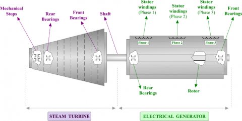
The steam turbine, rotor, stator, exciter, cooling system, and control system were all components of the turboalternator employed in this study. With a maximum rated output of 58 MW, the steam turbine was a single-stage impulse turbine. The stator held the coils of wire that generated the electrical output, while the rotor was constructed from several coils of wire wound around an iron core.
On the same shaft as the primary generator, the exciter was a generator that supplied enough electricity to induce a magnetic field in the rotor. A cooling tower and a heat exchanger were used in the cooling system, which used water cooling to remove heat from the steam turbine and the electrical generator.
The turboalternator's output and speed were controlled by the control system. Additionally, to controllers and other electronic components to adjust the steam flow rate and other parameters to maintain the desired output, it included sensors to measure various parameters like steam flow rate, steam pressure, and generator output.
The turboalternator was run continuously at 3000 RPM. A power analyzer, a pressure transducer, and a flow meter were just a few of the tools used to gather data daily.
The overall objective of the experimental setup was to test the performance of the system under various operating situations while simulating the real-world operating settings of a turboalternator.
Figure 1. Schematic sketch of the turboalternator
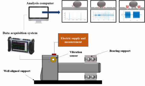
Figure 2. Process of data collection
The schematic sketch of the experimental testbed used to collect this data is shown in Figure 1.
Table 1 presents the nominal working conditions declared in the turboalternator machine manufacturer's guide.
Table 1. Nameplate of the studied turbogenerator
|
Parameter |
Nominal Value |
|
Active power |
58 MW |
|
Apparent power |
68 MVA |
|
Power factor |
0,85 |
|
Speed |
3000 rpm |
|
Voltage |
10 kV |
|
Phases |
3 |
|
Frequency |
50 Hz |
4.2 Data description
The data was acquired using a set consisting of a vibration sensor, a turbine, bearings, and an acquisition system. The first step was to make sure the acquisition system was ready to accept and record data from the vibration sensor and that it had been calibrated. The turbine's bearings were then fitted with the vibration sensor to measure vibration and temperature. The data were recorded using a sufficient sampling rate and resolution when the acquisition equipment was turned on. After starting the turbine, data was gathered for enough time (2 years), considering the frequency of potential problems and the necessary level of prediction accuracy. Figure 2 describes in detail the steps for data collection.
The recorded data was downloaded and kept in a secure location after data collection was finished to do additional analysis and processing. After collecting the data, it was evaluated to extract pertinent aspects and spot possible errors using the proper data processing and analysis procedures. Finally, depending on the recorded temperature and vibration levels, predictive models or algorithms that may detect and diagnose defects in the turbine bearings were created using the studied data.
In this section, the outcomes of our study evaluating the effectiveness of the three various training functions using the mean squared error (MSE) as the assessment metric are presented.
5.1 Levenberg Marquardt
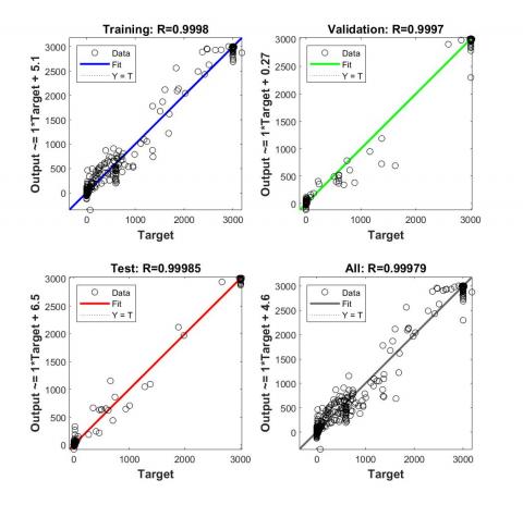
Figure 3 describes the regression model using Levenberg-Marquardt algorithm. The model fits the training data and the validation data very well with a regression coefficient respectively R= 0.9998 and R=0.9997, with a high degree of correlation between the predicted values and the actual values.
For the test data, we have R=0.99985, this means that the model is able to make accurate predictions on the test data as well.
Overall, these results suggest that the Levenberg-Marquardt algorithm had performed very well in fitting the model to the data, with high R values indicating a very good fit between the model and the observed data points.
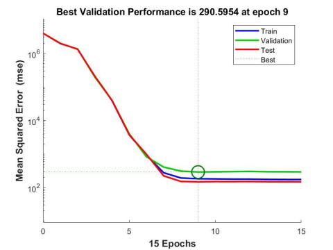
The Mean Squared Error (MSE) is a metric commonly used in the field of AI to quantify the average squared difference between predicted and actual values. It provides a measure of the overall accuracy of a predictive model by squaring the differences between predicted and observed outcomes, summing them, and then averaging across the dataset. MSE is particularly useful for regression tasks, helping assess how well a model's predictions align with the true values, with lower MSE values indicating better predictive performance. The MSE evolution over training (across various epochs) is shown in Figure 4. The best validation performance, as represented in the graph, was attained at epoch 9, which was a crucial stage in the training phase where the model's performance was optimized. These results indicate that the neural network was trained using the Levenberg-Marquardt method to produce moderately accurate predictions on the validation set, with the highest performance occurring at epoch 9.
Figure 3. Regression model using Levenberg-Marquardt algorithm
Figure 4. Evolution of the mean squared error (MSE)
Understanding the model's performance throughout the training phase and further optimizing it may benefit from this knowledge.
5.2 Bayesian regularization
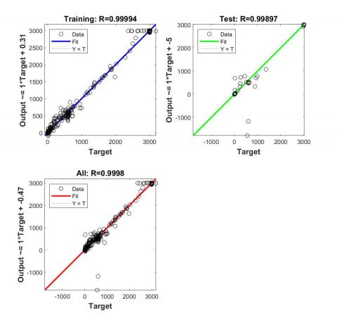
Figure 5 presents the regression model using Bayesian Regularization algorithm.
Figure 5. Regression model using Bayesian Regularization algorithm
For this model the training data has a regression coefficient respectively R= 0.9994. For the test data, we have R=0.99985.
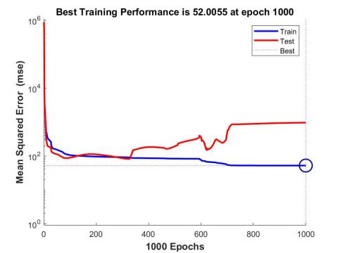
Figure 6. Evolution of the mean squared error (MSE)
As shown in the Figure 6 above, the best training performance was achieved at epoch 1000.
5.3 Scaled conjugate gradient
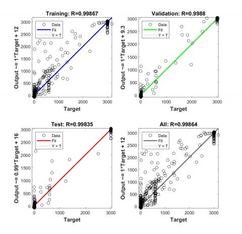
Figure 7 describes the regression model using Scaled conjugate gradient algorithm.
For the scaled conjugate gradient model, the training data and the validation had a regression coefficient respectively R= 0.99867 and R=0.9988. For the test data, we have R=0.99835.
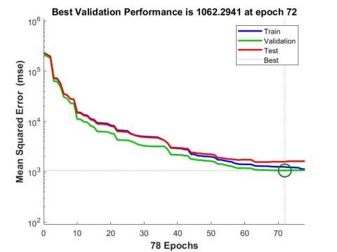
The best validation performance of the scaled conjugate gradient algorithm was achieved at epoch 72 shown in Figure 8. To analyze the three algorithms studied in the article, Table 2 presents a comparison between the results to choose the best among the three algorithms.
According to the values of the regression coefficients (Table 1), the tree algorithms appear to have done a great job of fitting the model to the data.
Figure 7. Regression model using scaled conjugate gradient algorithm
Figure 8. Evolution of the mean squared error (MSE)
Table 2. Technical comparison between the three algorithms
|
Algorithm |
Regression of the Training Data |
Regression of the Validation Data |
Regression of the Testing Data |
Regression of All |
|
Levenberg-Marquardt |
0.9998 |
0.9997 |
0.99985 |
0.99979 |
|
Bayesian Regularization |
0.99994 |
- |
0.99897 |
0.9998 |
|
Scaled Conjugate Gradient |
0.99867 |
0.9988 |
0.99835 |
0.99864 |
The results we obtained show that the output parameters of the turbogenerator set could be correctly predicted by all three training functions.
According to the results produced, the Bayesian Regularization approach had the lowest mean squared error (MSE) at epoch 1000 when comparing the performance of each training function over time. These findings imply that the Bayesian Regularization approach might be the best choice for forecasting the turbogenerator sets' output parameters.
The outcomes do, however, imply that the Bayesian Regularization technique was successful in instructing the neural network to make predictions that were essentially accurate, with high overall performance across all data points.
In this study, we evaluated the performance of three various ANN (artificial neural network) training functions when used on a turbogenerator set. The turbogenerator set provided the dataset for this study, which was made up of a variety of input and output parameters. In this study, Levenberg-Marquardt, Bayesian Regularization, and Scaled Conjugate Gradient were the three training functions employed. Based on the correlation coefficient (R) between the predicted and actual target values, each training function's performance was assessed.
The results of this study show the significance of choosing a suitable artificial neural network training function when forecasting the turbogenerator set output characteristics. In this work, the Bayesian Regularization approach performed the best overall, and our findings may be helpful in future research to optimize the performance of ANN models for turbogenerator sets.
The results of the article offer the possibility to:
The results of this study open several new research directions for example the use of linear SVM to predict To determine the optimal parameters. Examining how various artificial neural network training algorithms perform using the turbogenerator set dataset could be one possible topic of research. Furthermore, there were few input and output parameters included in the dataset used in this study. Future studies might examine how adding extra parameters affects how well ANN models work.
Examining the effectiveness of ANN models on different kinds of power producing machinery is another possible topic of research. It would be interesting to find out whether the results of this study generalize to other forms of power generation equipment as the turbogenerator set employed in this study is a particular sort of machinery.
Furthermore, although the correlation coefficient between the predicted and actual target values was used in this study to evaluate the performance of the ANN models, future research may investigate other metrics. For instance, if the models are being used for diagnostic or predictive purposes, it may be beneficial to investigate their sensitivity and specificity.
Overall, the results of this analysis show how artificial neural networks can be used to anticipate the turbogenerator sets' output characteristics and open up a number of new directions for further investigation.
[1] Patidar, S., Soni, P.K. (2013). An overview on vibration analysis techniques for the diagnosis of rolling element bearing faults. International Journal of Engineering Trends and Technology (IJETT), 4(5): 1804-1809.
[2] Nabhan, A., Ghazaly, N., Samy, A., Mousa, M.O. (2015). Bearing fault detection techniques-a review. Turkish Journal of Engineering, Sciences and Technology, 3(2): 1-18.
[3] Boudiaf, A., Moussaoui, A., Dahane, A., Atoui, I. (2016). A comparative study of various methods of bearing faults diagnosis using the case Western Reserve University data. Journal of Failure Analysis and Prevention, 16(2): 271-284. https://doi.org/10.1007/s11668-016-0080-7
[4] Dave, V., Singh, S., Vakharia, V. (2020). Diagnosis of bearing faults using multi fusion signal processing techniques and mutual information. Indian Journal of Engineering & Materials Sciences, 27(4): 878-888.
[5] Bonnardot, F., Randall, R.B., Antoni, J., Guillet, F. (2004). Enhanced unsupervised noise cancellation using angular resampling for planetary bearing fault diagnosis. International Journal of Acoustics and Vibration, 9(2): 51-60.
[6] Harsha, S.P., Nataraj, C., Kankar, P.K. (2006). The effect of ball waviness on nonlinear vibration associated with rolling element bearings. International Journal of Acoustics and Vibration, 11(2): 56-66.
[7] Sharma, A., Amarnath, M., Kankar, P.K. (2016). Feature extraction and fault severity classification in ball bearings. Journal of Vibration and Control, 22(1): 176-192. https://doi.org/10.1177/1077546314528021
[8] Wang, J., Cui, L., Wang, H., Chen, P. (2013). Improved complexity based on time-frequency analysis in bearing quantitative diagnosis. Advances in Mechanical Engineering, 5: 258506. https://doi.org/10.1155/2013/258506
[9] Kankar, P.K., Sharma, S.C., Harsha, S.P. (2011). Fault diagnosis of ball bearings using machine learning methods. Expert Systems with Applications, 38(3): 1876-1886. https://doi.org/10.1016/j.eswa.2010.07.119
[10] Samanta, B., Al-Balushi, K.R., Al-Araimi, S.A. (2003). Artificial neural networks and support vector machines with genetic algorithm for bearing fault detection. Engineering Applications of Artificial Intelligence, 16(7-8): 657-665. https://doi.org/10.1016/j.engappai.2003.09.006
[11] Zhang, X., Zhou, J. (2013). Multi-fault diagnosis for rolling element bearings based on ensemble empirical mode decomposition and optimized support vector machines. Mechanical Systems and Signal Processing, 41(1-2): 127-140. https://doi.org/10.1016/j.ymssp.2013.07.006
[12] Ali, J.B., Chebel-Morello, B., Saidi, L., Malinowski, S., Fnaiech, F. (2015). Accurate bearing remaining useful life prediction based on Weibull distribution and artificial neural network. Mechanical Systems and Signal Processing, 56-57: 150-172. https://doi.org/10.1016/j.ymssp.2014.10.014
[13] Das, O., Bagci Das, D. (2023). Smart machine fault diagnostics based on fault specified discrete wavelet transform. Journal of the Brazilian Society of Mechanical Sciences and Engineering, 45(1): 55. https://doi.org/10.1007/s40430-022-03975-0
[14] Sharma, A. (2022). Fault diagnosis of bearings using recurrences and artificial intelligence techniques. Journal of Nondestructive Evaluation, Diagnostics and Prognostics of Engineering Systems, 5(3): 031004. https://doi.org/10.1115/1.4053773
[15] Kaddari, M., Ennawaoui, C., Mouden, M.E., Hajjaji, A., Semlali, A. (2019). Diagnosis of shaft misalignment fault by piezoelectric materials to improve reliability of induction motors. International Journal on Engineering Applications, 7(4): 137-144.
[16] Wei, H., Zhang, Q., Shang, M., Gu, Y. (2021). Extreme learning Machine-based classifier for fault diagnosis of rotating Machinery using a residual network and continuous wavelet transform. Measurement, 183: 109864. https://doi.org/10.1016/j.measurement.2021.109864
[17] Yuan, H., Wang, X., Sun, X., Ju, Z. (2017). Compressive sensing-based feature extraction for bearing fault diagnosis using a heuristic neural network. Measurement Science and Technology, 28(6): 065018. https://doi.org/10.1088/1361-6501/aa6a07
[18] Sun, Y., Li, S. (2022). Bearing fault diagnosis based on optimal convolution neural network. Measurement, 190: 110702. https://doi.org/10.1016/j.measurement.2022.110702
[19] Patil, A.B., Gaikwad, J.A., Kulkarni, J.V. (2016). Bearing fault diagnosis using discrete wavelet transform and artificial neural network. In 2016 2nd International Conference on Applied and Theoretical Computing and Communication Technology (iCATccT), Bangalore, India, pp. 399-405. https://doi.org/10.1109/ICATCCT.2016.7912031
[20] Cui, B., Weng, Y., Zhang, N. (2022). A feature extraction and machine learning framework for bearing fault diagnosis. Renewable Energy, 191: 987-997. https://doi.org/10.1016/j.renene.2022.04.061
[21] Wagner, T., Sommer, S. (2020). Bearing fault detection using deep neural network and weighted ensemble learning for multiple motor phase current sources. In 2020 International Conference on INnovations in Intelligent SysTems and Applications (INISTA), Novi Sad, Serbia, pp. 1-7. https://doi.org/10.1109/INISTA49547.2020.9194618
[22] Vakharia, V., Gupta, V.K., Kankar, P.K. (2015). Ball bearing fault diagnosis using supervised and unsupervised machine learning methods. International Journal of Acoustics and Vibration, 20(4): 244-250.
[23] Wang, R., Jiang, H., Zhu, K., Wang, Y., Liu, C. (2022). A deep feature enhanced reinforcement learning method for rolling bearing fault diagnosis. Advanced Engineering Informatics, 54: 101750. https://doi.org/10.1016/j.aei.2022.101750
[24] Gao, S., Xu, L., Zhang, Y., Pei, Z. (2022). Rolling bearing fault diagnosis based on SSA optimized self-adaptive DBN. ISA Transactions, 128: 485-502. https://doi.org/10.1016/j.isatra.2021.11.024
[25] Sohaib, M., Kim, C.H., Kim, J.M. (2017). A hybrid feature model and deep-learning-based bearing fault diagnosis. Sensors, 17(12): 2876. https://doi.org/10.3390/s17122876
[26] Pham, M.T., Kim, J.M., Kim, C.H. (2020). Deep learning-based bearing fault diagnosis method for embedded systems. Sensors, 20(23): 6886. https://doi.org/10.3390/s20236886
[27] Ji, M., Peng, G., He, J., Liu, S., Chen, Z., Li, S. (2021). A two-stage, intelligent bearing-fault-diagnosis method using order-tracking and a one-dimensional convolutional neural network with variable speeds. Sensors, 21(3): 675. https://doi.org/10.3390/s21030675
[28] Beretta, M., Vidal, Y., Sepulveda, J., Porro, O., Cusidó, J. (2021). Improved ensemble learning for wind turbine main bearing fault diagnosis. Applied Sciences, 11(16): 7523. https://doi.org/10.3390/app11167523
[29] Liang, X., Yao, J., Zhang, W., Wang, Y. (2023). A novel fault diagnosis of a rolling bearing method based on variational mode decomposition and an artificial neural network. Applied Sciences, 13(6): 3413. https://doi.org/10.3390/app13063413
[30] Esakimuthu Pandarakone, S., Mizuno, Y., Nakamura, H. (2019). A comparative study between machine learning algorithm and artificial intelligence neural network in detecting minor bearing fault of induction motors. Energies, 12(11): 2105. https://doi.org/10.3390/en12112105
[31] Laayati, O., El Hadraoui, H., Guennoui, N., Bouzi, M., Chebak, A. (2022). Smart energy management system: Design of a smart grid test bench for educational purposes. Energies, 15(7): 2702. https://doi.org/10.3390/en15072702
[32] El Hadraoui, H., Zegrari, M., Hammouch, F.E., Guennouni, N., Laayati, O., Chebak, A. (2022). Design of a customizable test bench of an electric vehicle powertrain for learning purposes using model-based system engineering. Sustainability, 14(17): 10923. https://doi.org/10.3390/su141710923
[33] El Hadraoui, H., Laayati, O., El Maghraoui, A., Sabani, E., Zegrari, M., Chebak, A. (2023). Diagnostic and prognostic health management of electric vehicle powertrains: An empirical methodology for induction motor analysis. In 2023 5th Global Power, Energy and Communication Conference (GPECOM), Nevsehir, Turkiye, pp. 153-158. https://doi.org/10.1109/GPECOM58364.2023.10175674