Shubhangi Joteppa![]() | Santosh Kumar Balraj
| Santosh Kumar Balraj![]() | Nagamani Cheruku
| Nagamani Cheruku![]() | Tejesh Reddy Singasani
| Tejesh Reddy Singasani![]() | Venkateswarlu Gundu*
| Venkateswarlu Gundu*![]() | Aravinda Koithyar
| Aravinda Koithyar![]()
© 2024 The authors. This article is published by IIETA and is licensed under the CC BY 4.0 license (http://creativecommons.org/licenses/by/4.0/).
OPEN ACCESS
Chronic Kidney Disease (CKD) is often asymptomatic in its early stages, and patients may not experience noticeable symptoms until the disease has significantly progressed. This challenge in early detection results in patients seeking medical attention only when complications arise. Symptoms, when present, are nonspecific and vary widely among individuals, including fatigue, swelling, and changes in urination patterns, which may be mistakenly attributed to other conditions, leading to delayed diagnosis. In contemporary healthcare applications, the integration of Cloud Computing (CC) and the Internet of Things (IoT) has become commonplace. The cloud, with its superior processing capability compared to mobile devices, is particularly advantageous in analyzing the vast volumes of patient data generated by IoT devices. Machine Learning (ML) and Deep Learning (DL) models have gained interest in medical diagnostics due to their excellent prediction accuracy. This research introduces a novel method for diagnosing CKD using IoT and Cloud Computing. The selection of appropriate features and algorithms is crucial for optimizing the final model's performance. To address missing values and enhance results, a unique sequential approach is employed. Furthermore, the classification step utilizes m-Xception, employing a distinct architecture and breaking down the convolution layer into depth-based sub-layers linked by linear residuals. Effective model training results from a well-defined learning strategy. For selecting model kernel values, especially in large-scale examples, a Squeaky Wheel Optimization (SWO) metaheuristic is recommended. The projected model undergoes simulation testing on the canonical CKD dataset and is statistically evaluated. The findings suggest the feasibility of developing an automated method for estimating CKD severity. In conclusion, recent advances in predictive modeling and deep learning offer a fresh perspective on problem-solving, with potential applications in the field of renal illness and beyond.
min-max scaling, Internet of Things, CKD, Cloud Computing, kidney illness
The IoT is often used during the integration of software and hardware. Low-power applications, such as refrigerators, the like, have seen broad adoption of the Internet of Things, as opposed to high-power devices [1]. Only a few of today's air purifiers and air conditioners use a microprocessor and sensor devices. The Internet of Things (IoT) is making considerable strides towards full integration with the Cloud Computing (CC) paradigm, which has several advantages over traditional approaches [2]. Predicting Chronic Kidney Disease (CKD) using deep learning involves developing a model that can analyze relevant medical data and make predictions about whether a patient is likely to have CKD. Below is a high-level outline of the steps involved in building a deep learning model for CKD prediction: Advanced clinical and sensing equipment is desperately needed in medicine, which is one of the most promising disciplines [3, 4]. Early diagnosis and treatment of major diseases are becoming more challenging as the cost of medical equipment grows. To preserve a life, these measures are necessary. A web-based Clinical Decision Support System (CDSS) using IoT devices is suggested as a primary method for verifying the existence of life-threatening diseases in people [4]. Data science offers an essential way of capitalising on the quantity of information gathered by the Internet of Things for use in healthcare applications.
Healthcare monitoring systems, often known as e-Health systems, rely on wireless sensor networks (WSNs) [5]. Many of today's available smart watches boast of being able to track your health in minute detail. However, a medical diagnosis could not be made using one of these smartwatches. If a vital sign is off, only then will it provide a warning [6]. A dependable medical monitor is required here to track the patient's vitals. Devices such as blood pressure monitors, thermometers, heart rate monitors, electrocardiograms, pulse oximeters, and heart rate monitors are examples of medical equipment. Vital sign monitoring is a cornerstone of healthcare monitoring systems [7, 8]. Vital signs are monitored in the intensive care unit using healthcare monitoring systems [9]. That's why it's so significant to have healthcare monitoring systems in place for early disease detection [10]. A key drawback of healthcare monitoring systems has been the high upfront cost. The high expense of nations has created an urgent need for cost-effective healthcare solutions [11].
Constantly checking a patient's vitals might avert serious consequences from chronic diseases. When compared to other chronic illnesses, such as cardiovascular disease (CVD) or anaemia, chronic kidney disease is here cited as being more prevalent. The inability to produce enough erythropoietin hormones has been linked to a disease and anaemia in people with chronic kidney disease. Parameters including electrocardiogram (ECG), heart rate, and blood oxygen saturation monitoring may help in early detection [12]. These are some of the most common types of pollutants seen in ECG readings. Electrode are only some of the problems that might arise during an EMG recording [13]. Pollutants make it harder to interpret ECG readings, making it harder to diagnose heart problems. When kidneys are damaged to the point that they cannot filter blood properly and carry out other vital tasks, this is kidney disease (CKD). The medical term for the slow, progressive loss of kidney function that occurs over time is "chronic." CKD is a leading cause of death in countries owing to a lack of access to quality, cost-effective healthcare [14]. CKD may lead to cardiovascular disease and is permanent in its progression. In extreme circumstances, a kidney transplant or dialysis may be needed indefinitely. Early detection and treatment of chronic renal disease has been shown to enhance patients' quality of life [15]. Therefore, it is critical to detect and diagnose CKD early so that patients may start treatment immediately in an effort to arrest the progression of the disease [16].
Incorporating AI into medical monitoring devices will improve healthcare providers' decision-making. Machine learning is a cutting-edge method that shows promise for the accurate diagnosis and classification of many different medical conditions, including cardiovascular disease, cancer, renal failure, and stroke. This method has several applications outside of healthcare, including renewable energy generation [17]. Machine learning's (ML) use in healthcare has skyrocketed in recent years thanks to the proliferation of EMR big data [18]. Machine learning uses algorithms to analyse large datasets with many variables. Using ML prediction algorithms wisely may assist in the early, less costly treatment of many diseases. Therefore, it may be a workable strategy for detecting instances of CKD. Residual connections, inspired by ResNet (Residual Networks), can be beneficial in deep neural networks by alleviating the vanishing gradient problem and facilitating the training of very deep models. To incorporate ResNet-style residual connections into your model, you can modify the architecture of your deep learning model accordingly.
In order to predict CKD using DL approaches, this study contributes to the current literature by preprocessing the input dataset. The findings of this study would allow for the efficient and accurate management of known hazards in all contexts when doing so is practical and safe. The purpose of these methods is to help medical professionals classify disorders more precisely. In this work, we present a deep learning (DL) model that is trained on the UCI CKD dataset to enhance CKD diagnosis. The scalability of the perfect was improved by the use of missing-value imputation, scaling. Due to a lack of regularisation, Xception Net models might overfit their training data, resulting to inaccurate predictions and poor model evaluations when applied to fresh data. To address these concerns and prove the usefulness of log functions, the suggested model makes use of regularisation. In the m-Xception model, linear residuals link layers inside the convolution layer. Xception's classification accuracy may be improved by selecting the optimal kernel size with the help of the SWO model.
Here are the rest of the paper's chapters: This paper follows the following structure: There includes a literature review in Section 2, a brief explanation of the proposed model in Section 3, evaluations of the findings in Section 4, and a conclusion and swift in Section 5.
The beginning of chronic renal illness was predicted using a machine-learning model developed by Swain et al. [18] using publicly available data. This dataset underwent a battery of data grounding steps in order to construct a generic model. Before imputed values are created, the attributes are scaled and normalised using the SMOTE method. Using the fewest available observations, the chi-squared test establishes which features are essential and highly related to the output. Multiple supervised learning approaches are often integrated to construct a robust machine learning model. In comparison to other used learning strategies, support vector machine (SVM) the highest levels of test accuracy (99.33%) and false-negative rate (98.67%). However, when both methods were put through 10 rounds of cross-validation, SVM came out on top.
Alsekait et al. [19] presented a novel ensemble DL technique for identifying CKD by using several feature selection methods to zero in on the most informative features. We also look at how our best feature selection for CKD may be used in practise. To create the proposed ensemble model, we merge pre-trained deep learning models with the metalearner model, the support vector machine (SVM). UCI's machine learning repository supplied all 400 patients utilised in the research. The results validate the efficacy of the projected model in predicting CKD. The proposed model, which used the mutual_info_classi method to choose which features to utilise, performed the best.
Predicting and classifying CKD using ML techniques and a publicly accessible dataset was accomplished by Venkatesan et al. [20]. The CKD dataset, including 400 samples, was collected from the open-source Irvine ML Repository. eXtreme Gradient Boosting (XGBoost) is used to train the base learners, and the results are compared with those obtained using several other ML methods. The performance of ML algorithms may be evaluated using a variety of measures. The results shown that XGBoost achieved the highest accuracy (98.00%) when compared to the other ML algorithms. This study puts forward a methodology that might help policymakers estimate the global burden of CKD. The idea has the potential to facilitate better resource allocation, patient-centered care, and heightened surveillance of those at risk.
In order to diagnose and forecast the onset of CKD, Venkatrao and Kareemulla [21] created a novel HDLNet. As a deep learning-based strategy for CKD detection, the Deep Separable Convolution was suggested in this research. Capsule Network (CapsNet) may extrapolate processing quality from features known to indicate renal disease. By determining which characteristics are most important for classification, the Aquila Optimisation Algorithm (AO) helps to speed up the process. Classification efficiency is improved by the necessary qualities with just a little increase in processing effort. The DSCNN approach of classifying kidney illness into CKD and non-CKD is fine-tuned with the use of the Sooty Tern Optimisation is used for validation. Precision, recall, positive predictive value, are all measures of the efficacy of the optional CKD classification tactic. Further experimental data demonstrates that the suggested method outperforms the existing standard for CKD classification.
Dritsas and Trigka [22] came up with a plan to create accurate CKD prognostic tools using ML approaches. Before training and evaluating several ML models with different success measures, we employ class balancing to ensure an even distribution of cases across the two groups. In comparison to the other models used, Rotation Forest (RotF) achieved the highest levels of accuracy (99.2%), AUC (perfect), Precision (perfect), Recall (perfect), and F-Measure (perfect).
Combination the feature selection strategy with an AdaBoost classifier, Ebiaredoh-Mienye et al. [23] developed a method to correctly identify CKD. Since just a few number of clinical tests are needed to provide a diagnosis of CKD, this method of screening may be more cost-effective. The suggested strategy was compared to popular classifiers reduced feature set beat the other classifiers, 99.8% specificity. The feature selection was also shown to improve the presentation of the different classifiers in the experiments. The suggested method produced a reliable prediction model for CKD diagnosis and finding.
Abdel-Fattah et al. [24] propose a set of mixture machine learning strategies with the purpose of identifying CKD. In order to select the important features, the two techniques such as chi-squared and Relief-F were used in this work. Decision trees (DT), logistic regression (LR), Naive Bayes (NB), Boosted Trees (GBT Classifier) were all employed in this study as machine learning classification algorithms. Validation metrics included accuracy, precision, recall, and the F1-measure. Full features, Relief-F features, and chi-squared features have all been tested, and their respective cross-validation results have been determined. The findings demonstrated that using the chosen features led to the greatest performance for SVM, DT, and GBT Classifiers, achieving a perfect score of one hundred percent. By prioritising some traits above others, Relief-F achieves better results than either the whole set of features or the set of features.
2.1 Problem statement
A lifesaving CKD is essential. Experts in the medical field used numerous core methods, including physical exams and laboratory testing (including blood and urine tests), to get exact insights into renal disease diagnosis. The glomerular calculated from the blood sample, and it may be an indicator of kidney health. The albumin level in the urine is a good indicator of the health of the kidneys. Developing robust and generalizable diagnostic models that can support medical specialists and deliver correct and quick recommendations is essential in a time when promising data sources might aid in medical diagnosis. In the field of medical diagnostics, machine learning (ML) has recently helped build effective models that can make correct and fast choices. The goal of deep learning (DL), a subfield of machine learning, is to discover hidden relationships within a dataset by performing a series of operations during training. Medical applications are profoundly impacted by DL, a multilayer DL model that may, in theory, deal with nonlinear data.
The key to developing a powerful model is picking the right set of features to use. Extensive research on feature selection in the ML area has shown encouraging results in medicinal applications. Wrapper features, filter features, and embedded features are the three primary categories of feature options. In light of the above, this paper's primary goal is to refine DL in order to enhance prediction performance using the best possible collection of features. When compared to the current gold standard, our suggested feature list shows promise for early prediction of CKD from a clinical standpoint.
3.1 Dataset explanation
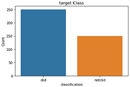
In this research, we used information from the UCI ML repository [25] to train our models. This collection is widely measured to be one of the best resources for machine learning datasets. This dataset contains 25 features across 400 records, including class attributes like CKD and NOTCKD to indicate whether or not a patient has CKD. This dataset includes both numerical features (eleven) and classified qualities (fourteen). There were several gaps in this data set; just 158 of the possible elements were filled out. There were 250 people diagnosed with CKD, compared to 150 people without the disease (37.5%). Table 1 summarises the most important information regarding the qualities.
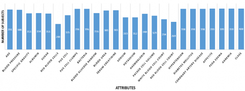
This research made use of information gathered on CKD.11 There are 14 rows and 400 columns in this data set. In the results, you'll see a "class" column with either "yes" or "no." In this case, the yes vote was worth one and the no vote was worth zero. Using the value "1" to indicate that the patient does really have CKD and the value "0" to indicate that they do not is common practise. Figure 1 displays the data set's properties.
There are about 250 people without CKD and just 140 people with CKD. Nearly 250 rows are CKD patients, whereas the remaining 150 rows are non-CKD affected role in the board class distribution (Figure 2).
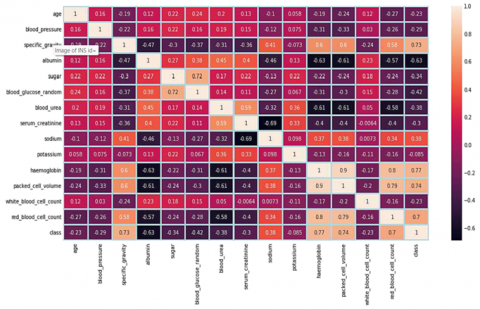
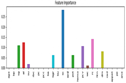
There are certain imbalances in the categorizations of some of the traits. Stratified folds are required for cross-validation. Absolute among the class label and features are shown in Figure 3 shows a data heatmap showing how the qualities are related to one another. Figure 4's heat map as positive associations among blood cell levels all have inverse relationships with one another.
Chronic renal disease affected 62.5% of the people in this research. In 37.5 percent of the samples, there is no detectable chronic renal disease. There is obviously no significant economic disparity between different populations. Figure 4 demonstrations the most notable features of the dataset.
Table 1. In-depth imageries of each chin in the chief CKD dataset
|
CKD Dataset |
Attributes Meaning |
Category |
|
al |
Albumin |
Nominal |
|
su |
Sugar |
Nominal |
|
rbc |
Red blood cells |
Nominal |
|
pc |
Pus cell |
Nominal |
|
pcc |
Not present, Present |
Category |
|
age |
Years |
Nominal |
|
bp |
mm/Hg |
Nominal |
|
sg |
1.005 to |
Nominal |
|
ba |
Not present, Present |
Nominal |
|
bu |
mgs/dl |
Nominal |
|
sc |
Blood serum |
Nominal |
|
pcv |
Hemoglobin |
Nominal |
|
wc |
Packed cell volume |
Nominal |
|
dm |
No, Yes |
Nominal |
|
cad |
No, Yes |
Nominal |
|
appet |
Poor, Good |
Nominal |
|
pe |
No, Yes |
Nominal |
|
Classification |
Not CKD |
Category |
Figure 1. Qualities in CKD dataset
Figure 2. Target class distribution
Figure 3. The heatmap of data with correlation profile
Figure 4. Significant features documentation from the dataset
3.2 Data preprocessing
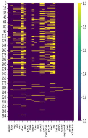
The preparation of the CKD dataset requires the elimination of outliers and the completion of missing data. The asymmetry in the dataset also introduces some bias. The preparation step [26] includes tasks like missing value estimation and imputation, noise removal (like outliers), and dataset rebalancing. As part of the definite features of the dataset were label-encoded to dummy values like 0 and 1. Figure 5 shows the extent to which our analysis revealed missing data.
Figure 5. The missing standards of the dataset
In the total dataset, only 158 patient records had no blanks. The missing information was filled in during the preprocessing stage, with the major imputation technique being the use of two median values. In the absence of outliers, the column mean (x) was used to infer missing values in numerical features. The centre was used for missing value charge in numerical features with outliers [27], since the imputed value would otherwise deviate from the average feature value range if x were used for imputation. Mo was used to fill in all of the blanks for the definite variables that were lacking data.
After imputation, the data were standardised. The dataset included 250 examples of patients with this ailment and 150 cases disorder, which led to the bias in the model. As such, a data-balancing method was included into the preparatory stage.
3.2.1 Data scaling
We begin by using resilient scaling, which mitigates the impact of extreme standards and increases the system's robustness. To achieve this, we took the difference between the third and second quartiles and divided it by the difference between the first and third quartiles (Q3 Q1). Here is the related equation:
$\operatorname{Robust} \operatorname{Scaling}(x)=\frac{x-Q_2}{Q_3-Q_1}$ (1)
After that, we employed z-score standardisation to produce a standardised distribution by subtracting the mean (m) and deviation (). Here is the related equation:
$Z-\operatorname{score}$ Standardization $(x)=\frac{x-\mu}{\sigma}$ (2)
Lastly, min-max scaling ($x_{\min }$) and in-between by the range ($x_{\max }-x_{\min }$). This can be characterised by the subsequent equation:
$\operatorname{Min}-\operatorname{Max} \operatorname{Scaling}(x)=\frac{x-x_{\min }}{x_{\max }-x_{\min }}$ (3)
3.2.2 Data excruciating
Accurate model evaluation and generalizability are essential for machine learning, and to achieve this, partitioning data is necessary [28, 29]. The first step is to divide the data into test and training sets.:
$Dataset = training\,\,data + testing\,\,data$ (4)
In this study, 80 percent of the data and 20 percent for testing. So, we train the model on a significant subset of the data and then put it through its paces on fresh data to see generalises.
3.3 Proposed model for classification
By substituting deep separable convolution for the original convolution in inception V3, the Xception network expands the network while simultaneously decreasing the amount of parameters and model computations. In addition, the network uses a ResNet-style residual connection technique to speed up convergence, improve classification accuracy, and fortify its ability to learn fine-grained features. Because it improves the representation's presentation without increasing network difficulty, this strategy is applicable to both CKD and normal classification. The model's convolution layer, which may be separated by depth, is connected with linear residuals. The network and is the foundation upon which the first flow is constructed. Separate convolution layers are used by the second flow, which is intermediate in nature. The core layer has been iterated upon eight times. The last stratum is exit circulation. This last layer is when the dense layer is formed. If "SWO" refers to an optimizer introduced after my last update or if it's a less well-known optimizer, I recommend checking recent literature, research papers, or official documentation from reputable sources to get the most accurate and up-to-date information.
If "SWO" is an abbreviation or acronym for a specific optimizer, it would be helpful to know the full name or context to provide a more accurate explanation.
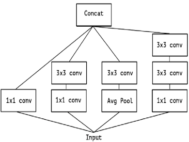
The Inception module has made this procedure more manageable and effective by breaking it down into a set of techniques that assess cross- correlations independently of one another. The Inception module was developed with the goal of improving the efficiency of the operation by assessing cross-channel correlations via the use of multiple 1 1 convolutions. Figure 6 shows how this works in practise: the input data is partitioned into three or four smaller areas, which are then convolutions, allowing for the charting of all correlations in the lesser 2D sectors.
Figure 6. The official Inception construction
By substituting deep separable convolution for V3, the Xception network expands the network while simultaneously decreasing the amount of parameters and model computations. In addition, the network uses a ResNet-style residual connection technique to speed up convergence, improve classification accuracy, and fortify its ability to learn fine-grained features. Because it recovers the model's presentation without increasing network complexity, this strategy is applicable to both CKD classification. The model's convolution layer, which may be separated by depth, is connected with linear residuals. The serves as a feature network and is the foundation upon which the first flow is constructed. Separate convolution layers are used by the second flow, which is intermediate in nature. The core layer has been iterated upon eight times. The last stratum is exit circulation. This last layer is when the dense layer is formed.
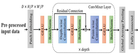
We've made an attempt to train dimensions, taking into account the physical dimensions as well as the convolution kernel, we simultaneously map spatial correlations. The Inception module has made this procedure more manageable and effective by breaking it down into a set of techniques that assess cross-channel and spatial correlations independently of one another. The Inception module was developed with the goal of improving the efficiency of the operation by assessing cross-channel correlations via the use of multiple 1 1 convolutions. Figure 7 shows how this works in practise: the input data is partitioned into three or four smaller areas, which are formerly convolutions, allowing 2D sectors.
Figure 7. Convolutional construction on DL
In this research, we use a convolutional construction on DL perfect as shown in Figure 7, where GELU represents for batch standardisation, H and W stand for kernel, P stands for kernels, and D is for the size of the input tensor.
In contrast to Normal Inception and Xception, which use an instantaneous ReLU function for non-linearity, the proposed model performs an 8X8 convolution. High performance is maintained experimentally without an instantaneous ReLU purpose, despite a modification in the order of operations. Compared to the existing convolution settings, this simplifies things without sacrificing speed.
Layer location and the basic sequence of convolution layers used to build the proposed Xception Net are shown in Figure 7. To simplify, the input tensor is subjected to the log (Softmax(x)) procedure.
$\begin{aligned} & \log S \text { of tmax }=\frac{\log (\exp (x))}{\sum \exp (x)} =x-\log \left(\left(\exp (x) \log \left(\sum \exp (x)\right)\right)\right)\end{aligned}$ (5)
The proposed model's loss function is optimised with the help of softmax of variable x. Over-fitting may be avoided during training thanks to a Regularise feature that regulates the layers.
Loss $=\frac{1}{n} \sum_1^n L_i+\lambda R w_i^2$ (6)
3.3.1 SWO-based heuristic outline
The SWO model is used to determine the optimal kernel size; the goal of the SWO-based heuristic approach is to hunt for keys in both the key space during the construction and priority phases, respectively. A solution to the issue may be thought of as a point in the solution space, and its related priority can be thought of as a point in space. The construction phase entails discovering a collection of potential solutions under the defined dispensation order for vessels, while the reassigning the order of vessels depending on their costs. The strategy focuses on prioritising the more costly vessels. To find the best answers, SWO iteratively adjusts the problem's priority and solution spaces.
A). Construction Phase
In (a), the sum of iterations is calculated. In we update the docking time to reflect the actual arrival time, with the beginning point being Vessel i's berthing position. If the number of quay cranes is more than q_imin, Step (d) allocates the sum of cranes to Vessel I so that it may be handled as rapidly as possible until Constraint (9) holds. If there are less than q_imin quay cranes available, as required by constraint (9), assignment of quay cranes must be discontinued. The berthing time for Vessel i may be delayed in Step (e), and then the quay crane task can be reallocated in Step (d), all without compromising the berthing position of Vessel i. If the delay is too lengthy, the process loops back to (c) to find a new place to dock the vessel. Due to the significant cost of horizontally relocating containers, there is a restriction on how far away the new berthing site may be from the previous one. (bi minus li plus li).
If the quay crane task is confirmed and one ship is booked in fee, then the completion time for Vessel i may be determined. map. If is to determine if delaying Vessel i or rerouting it to a different terminal would result in a cheaper overall cost. To finish placing the vessels, insert Vessel i′ next. In any other event, the current plan calls for reprocessing Vessel i's layout using the newest cohort of berthing locations. Once the berthing site and quay crane task for each vessel has been strongminded, the total cost may be calculated using function (1). Once the extreme sum of iterations has been reached, the process is restarted by returning to Step (a). In the conclusion, the construction step yields the most optimally identified vessel order.
B). Priority Phase
The purpose of phase is to identify a district arrangement that can handle the given order of boats. Select their objective values swap their order if the vessel contributes less to the total cost. If Vessel i is supplementary ahead of Vessel j and zj> zi, then the order of the vessels must be refigured. The goal of SWO is to focus those areas that offer the greatest percentage of the objective value by isolating these 'bottle neck' components and improving them as a top research priority. Therefore, the ship that accrued the most profit throughout its build should go to the front of the queue after the priority phase, and so on. Algorithm 1 provides a comprehensive description of the projected SWO perfect.
|
Algorithm 1: Over-all Outline of the Heuristic |
|
Input: baseline limits initialization; while the finish standards is not met do construction phase: get possible key $\left(b_i^i, C T_i^{\prime}, k_{i p}\right)$ calculate the separate cost $z^i$ $c_1 g_i\left|b_i-b_i^{\prime}\right|+c_0^i\left(C T_i^{\prime}-C T_i\right)+c_2 \sum_{j \in V} d_{i j} \lambda_{i j}$ priority phase: produce a novel instruction inse q' return: the negligeable cost of altogether vessels. end |
The Dell laptop was equipped with 16 GB of RAM, CPU, and Microsoft Windows 10 x64, and was utilised for all of the testing, analyses, and evaluations. We trained every network using the SWO optimizer for 10-30 iterations, and a focal loss function = 2. The learning degree was 1 x 10⁶ for the first 10 epochs, and then 1 x 10⁷ for the remaining 30 epochs.
4.1 Performance metrics
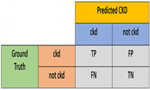
In this analysis, participants with CKD were given a positive value, whereas those without CKD were given a negative one. The results of the machine learning models were assessed and shown using matrix. The structure of a confusion matrix is seen in Figure 8 [30].
Figure 8. Confusion matrix
If the samples tested true positive (TP), then it was determined that they did in fact contain CKD. If the CKD trials provide a false-negative (FN) result, the diagnosis was incorrect. When samples are wrongly labelled as not originating from KD, this is known as a false-positive (FP) result. By definition, a "true negative," or "TN," means that the samples were appropriately identified as negative for CKD. [30]. Eqs. (7)-(11) provide the equations needed to determine them.
Accuracy $=\frac{T P+T N}{T P+F N+F P+T N}$ (7)
Recall $=$ Sentivity $=\frac{T P}{T P+F N}$ (8)
Specificity $=\frac{T N}{F P+T N}$ (9)
Precision $=\frac{T P}{T P+F P}$ (10)
$F 1$ score $=2 \frac{\text { precision } \times \text { recall }}{\text { precision }+ \text { recall }}$ (11)
4.2 Recital investigation of proposed approach
The Validation Analysis for the 80:20 model proposal is summarised in Table 2. The projected model achieved an F1-score of 98.16 and an accuracy of 97.56, with a precision degree of 98.33 and a recall range of 97.34. After those adjustments, the ResNet model achieved an F1-score of 94.38, precision of 89.33, recall of 94.64, and accuracy of 94.82. After those adjustments, the AlexNet model achieved an F1-score of 95.80, precision of 96.22, accuracy of 90.23, and recall of 96.67. As a result, the VGGNet model accomplished an F1-score of 97.33, recall range of 96.33, precision rate of 94.13, and accuracy of 94. 13.
Table 2. Validation analysis for the 80:20 model
|
Techniques |
Precision |
Recall |
F1-Score |
Accuracy |
|
ResNet |
89.33 |
94.64 |
94.38 |
94.82 |
|
AlexNet |
96.67 |
90.23 |
95.80 |
96.22 |
|
VGGNet |
95.33 |
96.33 |
97.33 |
94.13 |
|
Projected model |
98.33 |
97.34 |
98.16 |
97.56 |
Table 3 provides a summary of the classifier's performance on a number of different measures. In the study, the best implementation of the Decision Tree Classifier achieved a 0.983 accuracy in testing, 1.0 accuracy in training, 0.98 precision, 0.98 recall range, and 0.98 F1-score. Testing accuracy for the final CatBoost classifier was 0.975, accuracy was 0.98, precision was 0.98, recall range was 0.97, and the F1-score was 0.97. The KNN was then shown to be flawless, with a testing accuracy of 0.975, a accuracy of 0.985, a precision of 0.97, a recall range of 0.97, and an F1-score of 0.97. Finally, the F1-score for the Random Forest classifier was 0.59, as was the testing accuracy, the training accuracy, the precision, the recall range, and the F1-score. Next, the Naive Bayes classifier accomplished a flawless testing accuracy of 0.975, followed by a training accuracy of 0.99 within a range of 0.97, and an F1-score of 0.97. After reaching a accuracy of of 0.89, recall range of 0.88, and F1-score of 0.88, the Gradient boosting classifier was considered to be near-perfect. The LGBM classifier was then flawless, with a testing accuracy of 0.975, a training accuracy of 1.098, a precision of 0.97, and an F1-score of 0.97. The Extra tree classifier achieved a flawless F1-score of 0.975, precision of 0.98, recall within a range of 0.97, and accuracy of 0.975, 0.98, and 1.0 during training. Then, the SVM achieved a correctness of 0.983, a training of 0.98, recall within a range of 0.98, and an F1-score of 0.98. After reaching training accuracy of 1.0, testing accuracy of 0.9833, precision of 0.98, recall range of 0.98, and F1-score of 0.98, the ANN classifier was considered to be flawless. After that, we have ResNet at 0.9666, accuracy at 0.97, recall range at 0.97, then F1-score at 0.97. Thereafter, the AlexNet achieved a challenging accuracy of 0.6, a accuracy of 0.36, a recall range of 0.60, and an F1-score as 0.45. After reaching a training accuracy of 0.978, a testing accuracy of 0.958, a recall range of 0.96, and an F1-score as 0.96, the VGGNet was considered to be near-perfect. The proposed classifier reached an F1-scoree of 0.99 after achieving an accuracy of 0.9916 in testing, 0.946% in training, 0.946% to 0.99% in recall, and 0.99% to 99% in F1-score.
Table 3. Investigation of classifier on numerous systems of measurement
|
Classifiers |
F1-Score |
Training Accuracy |
Testing Accuracy |
Precision |
Recall |
|
Decision tree |
0.98 |
1.0 |
0.983 |
0.98 |
0.98 |
|
CatBoost |
0.97 |
0.98 |
0.975 |
0.98 |
0.97 |
|
Random forest |
0.59 |
0.76 |
0.59 |
0.58 |
0.59 |
|
ANN |
0.98 |
1.0 |
0.9833 |
0.98 |
0.98 |
|
ResNet |
0.97 |
0.946 |
0.9666 |
0.97 |
0.97 |
|
Naïve Bayes |
0.97 |
0.99 |
0.975 |
0.98 |
0.97 |
|
Gradient boosting |
0.88 |
0.9 |
0.8833 |
0.89 |
0.88 |
|
LGBM |
0.97 |
1.0 |
0.975 |
0.98 |
0.97 |
|
Extra tree |
0.97 |
1.0 |
0.975 |
0.98 |
0.97 |
|
SVM |
0.98 |
1.0 |
0.983 |
0.98 |
0.98 |
|
AlexNet |
0.45 |
0.6357 |
0.6 |
0.36 |
0.60 |
|
VGGNet |
0.96 |
0.978 |
0.958 |
0.96 |
0.96 |
|
Projected |
0.99 |
1.0 |
0.9916 |
0.99 |
0.99 |
Table 4. Investigation of innumerable classifiers on diverse epochs
|
Approaches |
10 Epochs |
30 Epochs |
|||||||
|
Train Acc. % |
Val. Acc. % |
Train Losses |
Val. Losses |
Train Acc. % |
Val. Acc. % |
Train Losses |
Val. Losses |
||
|
DBN |
75.6 |
75.4 |
88.14 |
88.41 |
73 |
71 |
83 |
82 |
|
|
m-Xception |
96.78 |
95 |
62.1 |
55 |
92 |
91 |
61 |
56 |
|
|
CNN |
83.24 |
84 |
73.1 |
71 |
81 |
79 |
81 |
75 |
|
|
ResNet |
87.1 |
87 |
74 |
77 |
80 |
72 |
73 |
80 |
|
|
VGGNet |
94.11 |
95.32 |
71 |
73 |
82 |
81 |
79 |
72 |
|
|
AlexNet |
88.54 |
88 |
89 |
82 |
81 |
78 |
77 |
75 |
|
|
RNN |
82 |
82 |
76.44 |
73 |
76 |
75 |
85 |
81 |
|
Table 4 above shows the examination of numerous classifiers throughout many time periods. Training accuracy for the DBN model was 75.6%, validation accuracy was 75.4%, and loss for training was 88.14% and loss for validation was 88.51% during the course of the 10-epoch study. The RNN model accomplished an accuracy of 82 during training, an accuracy of 82 during validation, a training loss of 76.44, and a validation loss of 73. The final results for the CNN model were an accuracy of 83.24 in training, 84 in authentication, a loss of 73.1 in training, and 71 in validation. The ResNet model eventually reached an 87.1 accuracy during training, an 87.5 accuracy during validation, and a validation loss of 77. Training accuracy for the AlexNet model was 88.54 percent, validation correctness was 88 percent, training loss was 89 percent, and validation loss was 82 percent. The final results for the VGGNet model were a 94.11 percent training accuracy, a 97.17 percent validation accuracy, and a 95.32 percent training loss. After then, the m-Xception perfect accomplished 96.78% in accuracy, 95% in loss, and 55.1% in validation loss. Following an additional 30-epoch examination, the DBN perfect achieved an accuracy of 88.14 during training, an accuracy of 89.5 during validation, a loss of 88.41 during training, and a loss of 82.0 during validation. The final results for the RNN model were an accuracy of 76.44 in training, an accuracy of 73.76 in validation, a loss as 75.85 in training, and a loss as 81 in validation. The final results for the CNN model were an accuracy in training of 73.1, an accuracy in validation of 71, and a loss in training of 81, 79, and 81. Training accuracy for the ResNet model was 74, validation accuracy was 77, and training loss was 80. After that, the AlexNet model achieved an accuracy of 89 in training, 82 in validation, 81 in loss in training, 78 in loss in validation, and 75 in loss in validation. Training accuracy for the VGGNet model was 71, authentication accuracy was 73, loss during training was 82, loss during validation was 81, loss during validation was 79, and loss during validation was 72. Training accuracy for the m-Xception model was 62.1, whereas validation accuracy was 55.92, training loss was 91, and validation loss was 61, and authentication loss was 56.
Managing chronic renal disease poses a significant medical challenge. Early detection of chronic kidney disease (CKD) can substantially benefit individuals suffering from it. Patient records included in this analysis were gathered over a two-month period. Utilizing data from a diverse group of real-world patients, this research investigates the feasibility of CKD prediction, achieving a very high accuracy of 99.0 percent. This accuracy is instrumental in the early identification of renal illness. The proposed approach replaces the Inception classification module used in mobile net with an m-Xception-residual model. However, the projected model incorporates a logarithmic-based softmax layer to extract classification features, contributing to an increased accuracy rate in making precise predictions. The optimal kernel size is determined by the SWO method. The results indicate that the recommended approach achieved a success rate of 96.78% on the 10th epoch and 92% on the 30th epoch. Utilizing the proposed models in resource expansion, patient monitoring, and early CKD diagnosis has demonstrated positive benefits in our study. Future research of this nature should involve more comprehensive datasets, including data from a broader demographic range. It should explore additional relevant features that could contribute to CKD prediction and consider collaboration with domain experts and healthcare professionals to identify and incorporate valuable features.
[1] Hosseinzadeh, M., Koohpayehzadeh, J., Bali, A.O., Asghari, P., Souri, A., Mazaherinezhad, A., Bohlouli, M., Rawassizadeh, R. (2021). A diagnostic prediction model for chronic kidney disease in internet of things platform. Multimedia Tools and Applications, 80: 16933-16950.
[2] Burgos-Calderón, R., Depine, S. Á., Aroca-Martínez, G. (2021). Population kidney health. A new paradigm for chronic kidney disease management. International Journal of Environmental Research and Public Health, 18(13): 6786. https://doi.org/10.3390/ijerph18136786
[3] Venkateswara Rao, M., Sreeraman, Y., Mantena, S.V., Gundu, V., Roja, D., Vatambeti, R. (2024). Brinjal Crop yield prediction using shuffled shepherd optimization algorithm based ACNN-OBDLSTM model in smart agriculture. Journal of Integrated Science and Technology, 12(1): 2321-4635. https://pubs.thesciencein.org/journal/index.php/jist/article/view/a710/423
[4] Chan, A.S.W., Ho, J.M.C., Li, J.S.F., Tam, H.L., Tang, P. M.K. (2021). Impacts of COVID-19 pandemic on psychological well-being of older chronic kidney disease patients. Frontiers in Medicine, 8: 666973. https://doi.org/10.3389/fmed.2021.666973
[5] Macherla, H., Kotapati, G., Sunitha, M.T., Chittipireddy, K.R., Attuluri, B., Vatambeti, R. (2023). Deep learning framework-based chaotic hunger games search optimization algorithm for prediction of air quality index. Ingénierie des Systèmes d’Information, 28(2): 433-441. https://doi.org/10.18280/isi.280219
[6] Srivastava, S., Yadav, R.K., Narayan, V., Mall, P.K. (2022). An ensemble learning approach for chronic kidney disease classification. Journal of Pharmaceutical Negative Results, 2401-2409. https://www.pnrjournal.com/index.php/home/article/view/9054/12404.
[7] Inamanamelluri, H.V.S.L., Pulipati, V.R., Pradhan, N.C., Chintamaneni, P., Manur, M., Vatambeti, R. (2023). Classification of a new-born infant’s jaundice symptoms using a binary spring search algorithm with machine learning. Revue d'Intelligence Artificielle, 37(2): 257-265. https://doi.org/10.18280/ria.370202
[8] Wilkinson, T.J., Miksza, J., Yates, T., Lightfoot, C.J., Baker, L.A., Watson, E.L., Zaccardi, F., Smith, A. C. (2021). Association of sarcopenia with mortality and end‐stage renal disease in those with chronic kidney disease: A UK Biobank study. Journal of cachexia, sarcopenia and muscle, 12(3): 586-598. https://doi.org/10.1002/jcsm.12705
[9] Campbell, Z.C., Dawson, J.K., Kirkendall, S.M., McCaffery, K.J., Jansen, J., Campbell, K.L., Lee, V.W., Webster, A.C. (2022). Interventions for improving health literacy in people with chronic kidney disease. Cochrane Database of Systematic Reviews, 2(12):CD012026. https://doi.org/10.1002/14651858.cd012026.pub2
[10] Senan, E.M., Al-Adhaileh, M.H., Alsaade, F.W., Aldhyani, T.H., Alqarni, A.A., Alsharif, N., Uddin, M.I., Alahmadi, A.H., Jadhav, M.E., Alzahrani, M.Y. (2021). Diagnosis of chronic kidney disease using effective classification algorithms and recursive feature elimination techniques. Journal of Healthcare Engineering, 2021: 1004767. https://doi.org/10.1155/2021/1004767
[11] Banik, S., Ghosh, A. (2021). Prevalence of chronic kidney disease in Bangladesh: A systematic review and meta-analysis. International Urology and Nephrology, 53: 713-718. https://doi.org/10.1007/s11255-020-02597-6
[12] Bai, Q., Su, C., Tang, W., Li, Y. (2022). Machine learning to predict end stage kidney disease in chronic kidney disease. Scientific reports, 12(1): 8377.
[13] Debal, D.A., Sitote, T.M. (2022). Chronic kidney disease prediction using machine learning techniques. Journal of Big Data, 9: 109. https://doi.org/10.1186/s40537-022-00657-5
[14] Gulamali, F.F., Sawant, A.S., Nadkarni, G.N. (2022). Machine learning for risk stratification in kidney disease. Current Opinion in Nephrology and Hypertension, 31(6): 548-552. https://doi.org/10.1097/mnh.0000000000000832
[15] Gunapriya, B., Rajesh, T., Thirumalraj, A., Manjunatha, B. (2023). LW-CNN-based extraction with optimized encoder-decoder model for detection of diabetic retinopathy. Journal of Autonomous Intelligence. 7(3). https://doi.org/10.32629/jai.v7i3.1095
[16] Asniar, Maulidevi, N.U., Surendro, K. (2022). SMOTE-LOF for noise identification in imbalanced data classification. Journal of King Saud University - Computer and Information Sciences, 34: 3413-3423. https://doi.org/10.1016/j.jksuci.2021.01.014
[17] Krishnamurthy, S., Ks, K., Dovgan, E., Luštrek, M., Gradišek Piletič, B., Srinivasan, K., Jack Li, Y.C., Gradišek, A., Syed-Abdul, S. (2021). Machine learning prediction models for chronic kidney disease using national health insurance claim data in Taiwan. In Healthcare, 9(5): 546. https://doi.org/10.3390/healthcare9050546
[18] Swain, D., Mehta, U., Bhatt, A., Patel, H., Patel, K., Mehta, D., Acharya, B., Gerogiannis, V.C., Kanavos, A., Manika, S. (2023). A robust chronic kidney disease classifier using machine learning. Electronics, 12(1), 212.
[19] Alsekait, D.M., Saleh, H., Gabralla, L.A., Alnowaiser, K., El-Sappagh, S., Sahal, R., El-Rashidy, N. (2023). Toward comprehensive chronic kidney disease prediction based on ensemble deep learning models. Applied Sciences, 13(6): 3937. https://doi.org/10.3390/app13063937
[20] Venkatesan, V.K., Ramakrishna, M.T., Izonin, I., Tkachenko, R., Havryliuk, M. (2023). Efficient data preprocessing with ensemble machine learning technique for the early detection of chronic kidney disease. Applied Sciences, 13(5): 2885. https://doi.org/10.3390/app13052885
[21] Venkatrao, K., Kareemulla, S. (2023). HDLNET: A hybrid deep learning network model with intelligent IoT for detection and classification of chronic kidney disease. IEEE Access, 11. https://doi.org/10.1109/ACCESS.2023.3312183
[22] Dritsas, E., Trigka, M. (2022). Machine learning techniques for chronic kidney disease risk prediction. Big Data and Cognitive Computing, 6(3): 98. https://doi.org/10.3390/bdcc6030098
[23] Ebiaredoh-Mienye, S.A., Swart, T.G., Esenogho, E., Mienye, I.D. (2022). A machine learning method with filter-based feature selection for improved prediction of chronic kidney disease. Bioengineering, 9(8): 350. https://doi.org/10.3390/bdcc6030098
[24] Abdel-Fattah, M.A., Othman, N.A., Goher, N. (2022). Predicting chronic kidney disease using hybrid machine learning based on apache spark. Computational Intelligence and Neuroscience, 2022:9898831. https://doi.org/10.1155/2022/9898831
[25] UCI Machine Learning Repository. Chronic Kidney Disease Dataset. Available online: https://archive.ics.uci.edu/ml/datasets/ chronic_kidney_disease, accessed on 11 Dec. 2022.
[26] Kotsiantis, S., Kanellopoulos, D., Pintelas, P. (2016). Handling imbalanced datasets: A review. G https://www.researchgate.net/publication/228084509_Handling_imbalanced_datasets_A_review
[27] Audu, A., Danbaba, A., Ahmad, S.K., Musa, N., Shehu, A., Ndatsu, A.M., Joseph, A.O. (2021). On the efficiency of almost unbiased mean imputation when population mean of auxiliary Variable is Unknown. Asian Journal of Probability and Statistics, 15: 235-250. http://dx.doi.org/10.9734/AJPAS/2021/v15i430377
[28] Joseph, V.R. (2022). Optimal ratio for data splitting. Statistical Analysis and Data Mining: The ASA Data Science Journal, 15: 531-538. https://doi.org/10.1002/sam.11583
[29] Chollet, F. (2017). Xception: Deep learning with depthwise separable convolutions. In Proceedings of the IEEE Conference on Computer Vision and Pattern Recognition, Honolulu, HI, USA, pp. 1251-1258. https://doi.org/10.1109/CVPR.2017.195
[30] Rácz, A., Bajusz, D., Héberger, K. (2019). Multi-level comparison of machine learning classifiers and their performance metrics. Molecules, 24(15): 2811. https://doi.org/10.3390/molecules24152811