Remesh Kollezhath Muraleedharan*![]() | Latha Ravindran Nair
| Latha Ravindran Nair![]()
© 2024 The authors. This article is published by IIETA and is licensed under the CC BY 4.0 license (http://creativecommons.org/licenses/by/4.0/).
OPEN ACCESS
Three-way decisions play a crucial role in addressing decision-making problems in situations of uncertainty. They categorize the decision space into three discrete regions, specifically referred to as the Positive, Negative, and Boundary regions. These models are frequently employed in scenarios that involve the existence of multiple potential alternatives, necessitating the inclusion of a deferral option in addition to the two extremes. This methodology is especially advantageous in situations where the intricacy of the decision-making environment necessitates a more sophisticated examination of potential options that extend beyond a binary choice. The concept of information granularity is the foundation for the ability to conceptualize, comprehend, and apply a sequential three-way decision approach. When working with fine-grained granules, people have the freedom to carefully consider all of their options before deciding on any one. The application of sequential three-way decisions results from the availability of detailed information. Through the application of various techniques and a shift from coarse to fine-grained information granularity, this decision-making method establishes specific thresholds for efficient decision-making. This study introduces an innovative approach for exploring objects that have not made a definitive decision ultimately leading to the convergence of these objects into the Positive and Negative regions. The Chi-square statistic is employed as the evaluative measure for the process of dividing the decision space into three distinct regions.
granular computing, sequential three-way decisions, TAO model, Chi-square statistic, objective functions, optimal thresholds
The dynamic and swiftly evolving field of granular computing in data processing has garnered significant interest from both academics and industry experts. The term "granular computing" refers to a broad category of speculations, methods, processes, and tools that employ information granules to address complex problems.
One of the most fastly expanding paradigms for data processing is granular computing, which has found a home in the fields of AI and human-centered systems.
The concept of "thinking in threes" serves as the foundation for three-way decisions (TWD). The strategy is based on in-depth research into the cognitive, learning, and decision-making processes of people. Trisecting and acting are two tasks that are intertwined in making TWDs [1]. The TAO (trisecting-acting-outcome) model of TWD partitions the entire thing into three logical slices. The effectiveness of the result is then evaluated, and a corresponding strategy is created. Figure 1 depicts the TAO model in its most basic form.
At Level 1, Universe, which stands for the "Whole," represents all of the characteristics, actions, or other things that make up the entire collection of objects [2, 3]. Universe is divided into three separate and non-overlapping parts, namely Part I, Part II, and Part III, which are referred to as level 2 components such that components such that PartI U PartII U PartIII $=$ Universe and PartI $\cap$ PartII $=\Phi$, Part $I I \cap$ Part $I I I=\Phi$, PartI $\cap$ Part $I I I=\Phi[2]$. During the phase of 'Acting', the decision-maker is required to develop a strategic plan of action and implement it to achieve the desired outcome [2]. The success of the TAO model relies on the efficient alignment of trisecting methods and strategies for actions, which presents a significant challenge in the domain of three-way decisions [2].
Figure 1. The TAO model
The notion of diminishing boundary areas has emerged as a contemporary advancement in the sequential three-way decision-making process. Real-world decision-making allows for the consideration of multiple points of view, which ultimately results in two-way decisions. More new information is learned with each view. A new approach, based on the idea of granularity in multiple perspectives, is presented in this paper. Various granularity levels are represented by different subsets of the sample's total attribute set. Granules can be thought of as a metaphor for any kind of collection, grouping, classification, clustering, or set of ideas or objects [3]. The granular structure is made up of granules that are all roughly the same granularity and shape. There are many different features and connections within the structure that can be brought to light by using a finer granularity. Since the granular structure's levels are organized hierarchically based on the level of detail they contain, the structure of information features and relationships is generated hierarchically. By conducting investigations at different levels of granularity, one can obtain different types of knowledge and understand the underlying constitution of the accumulated knowledge [4, 5].
In practical decision-making scenarios, it is common to encounter a sequence of three-way decisions that eventually lead to two-way decisions. At every point of decision, further and more comprehensive data is acquired. In the context of clinical decision-making, a physician may opt to administer treatment or abstain from doing so for specific patients, relying on available data. In certain cases, the physician may suggest conducting supplementary examinations and deferring a determination until the subsequent phase [2, 6].
The creation of a multi-level granularity sequence for TWD is the first significant challenge. Partially ordered informational granularity, or multi-granulation provides the semantics for the Sequential Three-way Decision (STWD) model [7]. The interpretation of STWD evaluations and thresholds is the second issue, and the introduction of the objective function to select the best thresholds for trisection is the third but the most significant problem. Possible interpretations of objective functions could include various factors, including considerations of costs, benefits, information entropy, and desirability.
The subsequent sections of this paper are structured as follows. Section 2 gives a fundamental idea about granular computing.Section 3 of the study focused on sequential three-way decisions and their hierarchical structure and delved into the concept of information granularity. In Section 4, the Chi-square statistic was utilized as the objective function and a novel approach was introduced to determine the optimal threshold values. Section 5 validates the experimental findings and concludes the paper in Section 6.
2.1 Granules
Granules are the fundamental components of computing on a granular level. According to the definition given in Merriam-Webster’s Dictionary [8], a granule is "a small particle; especially, one of many particles forming a larger unit". Any universe's subsets, classes, objects, clusters, and elements that can be grouped based on distinguishability, similarity, or functionality are granules [9-11]. A subset, a class of the universe that is equivalent, a paragraph, an interval of a universe, and a system module are examples of granules [9].
Sub-granules, which are smaller or finer versions of these granules, are capable of further decomposition. Granules can be graded based on complexity, level of abstraction, and size. At the largest and coarsest granule, the problem domain or the universe exists. The most fundamental particles or elements of the specific model being used make up granules at the lowest level [9].
2.2 Granulation
One of the major problems with using granular computing to solve problems is granulation. It is the process of constructingor decomposinggranules. Granulation could be described as the process that involves both construction and decomposition when solving problems. By combining smaller sub-granules, a larger, more complex granule can be built. The decomposition process involves the fragmentation of a larger granule into numerous smaller granules at progressively lower stages [9, 10].
2.3 Relationships
It is impossible to perform granulation without first establishing the relationships between the granules, as these relationships serve as the basis for either fusing smaller granules to form larger ones or crushing larger granules into smaller ones at various levels. The relationships at the granular level can be classified as either intra or inter. In decomposition, a large-sized granule is broken down into a small one capable of being put to use even then to make another larger granule. Construction is the process of assembling smaller granules that are functionally and aesthetically comparable to larger granules. The relationship present in the former granulation is referred to as an inter-relationship, whereas it is an intra-relationship in the latter. In other words, the intra-relationship is the basis for breaking a granule into smaller pieces, whereas the inter-relationship is the basis for grouping small objects [6].
Sometimes, in the real world, you have to make a series of three-way decisions before you settle on a two-way one. New and more information is gathered at each stage. For instance, a physician making a clinical decision may choose to treat a patient or not to treat a patient based on the available data, while deciding for another patient may be delayed by recommending further testing [12]. Models of STWD with probabilistic rough sets and Wald's sequential three-way hypothesis testing model share many of the same core ideas [12].
A formalization of STWD can be achieved through the use of the concept of multiple levels of granularity [13-15]. Let there be n +1 granularity levels with n>=1. Indices 0, 1, 2,..., n are used to represent the n+1 levels to keep things simple, with 0 standing for the highest degree of granularity (i.e., the bottom stage) and n for the most coarse-grained. Level 0 decision-making can be thought of as simple two-way decisions. For STWD with n levels, three-way decisions are done at all the levels n, n-1,..., 1, and made a two-way decision at level 0. To rephrase, a series of three-way choices leads to a two-way choice [12].
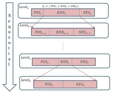
By combining a granular computing perspective with three-way decisions, Yao showed that they are a powerful solution from the perspective of multi-granulation [12, 15]. In addition, Yao put forth a generic model for making STWD. Users can tailor the STWD definition for this overarching model to their specific needs, using the applications and data at hand. Use this model to specify how to go from boundary decisions made initially, to a set of decisions either positive or negative [12].
Figure 2. STWD model
The fundamental structure of an STWD model is given in Figure 2. The number of granularity levels is n+1 (n ≥1). U is factored into three different fractions at the top level (level n), i.e., Un=POSn U BNDn U NEGn. In general, BNDi+1 is factored into three fractions for level i (1<= i <=n-1); thus, BNDi+1=POSi U BNDi U NEGi. BND1 is finally factored into two regions that are pairwise separable for level 0, i.e., BND1=POS0 U NEG0 [15].
In practical scenarios, it is frequently observed that decision-makers often encounter a scarcity of comprehensive information. In instances of this nature, a prompt and economical determination can be rendered, yielding an approximate yet potentially hazardous outcome. The decision model illustrated in Figure 2 follows a sequential three-way approach, guided by the concept of granularity. This approach involves progressing from the broadest level of granularity to the most detailed level. STWD is designed to offer a more adaptable mechanism for making decisions, which gradually incorporates more fine-grained data. A sequential process that moves from broad strokes to pinpoint details enables users to make better decisions. The STWD process is more effective than the TWD with time and money as it takes less time and uses less information than the TWD does [16, 17]. Taking this approach, which is representative of human thought and choice, yields the STWD model [1, 7, 15, 18].
For sequential three-way decisions, the following semantic concerns must be addressed: (1) building and interpreting a hierarchy of granularity levels, and (2) building and interpreting the objective function and thresholds (α, β) for each granularity level [15].
The universe can be thought of as a collection of information granules, each of which provides information about a narrow facet of a system or problem. The degree of generalization or abstraction that some information provides can be interpreted as the granularity of a granule. By collecting granules of the same granularity, we can obtain a comprehensive description of a system or problem. The collection of granules encapsulates the granulation of the issue at a specific level [15, 19, 20].
Typically, an object's equivalence class [x]A serves to describe it. Assume that A=a1, a2,..., an is a set of attributes and that A1={a1, a2,..., an}, A2={a1, a2,..., an-1}, …….. An={a1} respectively. Then, attribute sets can be obtained due to equivalence classes regarding the granularity structure's design {A1, A2,..., An}. By sorting the attributes by significance, costs, etc., a wide range of granularity structures can be constructed to tackle a wide range of problems [15].
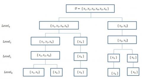
Constructing classes of x having equivalence with the number of attributes increasing is required to make a coarsening-refining granularity family on information granules. Four granules of each of the objects in Table 1 produced a chained equivalence relation set that led to the multilevel partition depicted in Figure 3.
As shown in Figure 3, there are four levels of granularity in the granularity structure for Table 1 . A granule in the $i^{\text {th }}$ level is denoted as $\left(A_i\right), 1 \leq i \leq 4$. The granulation at each level is represented as [15]:
$\begin{aligned} & \text { level 3, } G_{U / A_4}=g\left(\left\{a_1\right\}\right)=\left\{\left\{x_1, x_2, x_4, x_6\right\},\left\{x_3, x_5\right\}\right\} \\ & \text { level 2, } G_{U / A_3}=g\left(\left\{a_1, a_2\right\}\right)=\left\{\left\{x_1, x_2, x_6\right\},\left\{x_3, x_5\right\},\left\{x_4\right\}\right\} \\ & \text { level1, } G_{U / A_2}=g\left(\left\{a_1, a_2, a_3\right\}\right)= \left\{\left\{x_1, x_2, x_6\right\},\left\{x_3\right\},\left\{x_4\right\},\left\{x_5\right\}\right\} \\ & \text { level 0, } G_{U / A_1}=g\left(\left\{a_1, a_2, a_3, a_4\right\}\right)= \left\{\left\{x_1, x_2\right\},\left\{x_3\right\},\left\{x_4\right\},\left\{x_5\right\},\left\{x_6\right\}\right\}\end{aligned}$
Sequential three-way decisions have practical applications in a wide range of real-world scenarios. In the field of healthcare, medical professionals frequently engage in the process of making sequential three-way decisions about the treatment of patients. The initial decisions may encompass the determination of whether to promptly administer treatment, postpone treatment while awaiting additional diagnostic tests, or opt for no treatment. In the case of financial investments, Investors may employ a sequential three-way decision-making approach in the management of investment portfolios. Investors make decisions regarding the retention, divestment, or acquisition of supplementary investments in response to fluctuating market dynamics and the availability of new information [17, 21-23]. In the domain of supply chain operations, decision-makers often employ a sequential three-way decision framework to ascertain whether it is appropriate to initiate an immediate inventory reorder, postpone the decision until more market information becomes available, or explore alternative suppliers as a viable option.
Table 1. Decision table
|
|
a1 |
a2 |
a3 |
a4 |
D |
|
x1 |
1 |
0 |
1 |
1 |
d1 |
|
x2 |
1 |
0 |
1 |
1 |
d2 |
|
x3 |
0 |
1 |
0 |
1 |
d3 |
|
x4 |
1 |
1 |
0 |
0 |
d4 |
|
x5 |
0 |
1 |
1 |
0 |
d5 |
|
x6 |
1 |
0 |
1 |
0 |
d6 |
By representing the boundary region as a granule, it becomes feasible to progressively divide the boundary region into different levels until a binary division is attained. This innovative technique has the potential to be applied in practical situations, especially when decision-making becomes more difficult due to uncertainty. It offers an alternative and effective way to improve the decision-making process.
Figure 3. Hierarchical granularity structure
The creation of the granularity structure employs a novel concept. This research proposes a new method for finding the optimal threshold values by using Chi-square statistics to divide the decision space into three distinct regions: the Positive, the Negative, and the Boundary. The boundary region's objects are once again divided into three regions as described before, using the Chi-square statistics as the objective function, and two new ideal thresholds are determined while treating the boundary region as the universe. This process is carried out repeatedly until the boundary region is empty. Consequently, an STWD model can be constructed with granularities ranging from the most general to the most specific.
4.1 The use of Chi-square statistics for deciding between three alternatives
Objects in the universe $U$ are divided into two groups $\left\{C, C^C\right\}$, with $C$ representing the object set in the class and $C^C$ representing the object set that does not belong to it, and $C \cup C^C=U$. The evaluation function trisects the universe $U$ into three regions using two thresholds $(\alpha, \beta)$ namely $P O S_{(\alpha, \beta)}(C), B N D_{(\alpha, \beta)}(C), N E G_{(\alpha, \beta)}(C)$ respectively, as an approximation of $\left\{C, C^C\right\}$ [23, 24].
The quality or goodness of trisection is measured by an objective function that can be formulatedby a linearcombination ofthe qualities of the three regions as [25]:
$Q\left(\pi_{(\alpha, \beta)}(C)\right)=w_1 Q_P(\alpha, \beta)+w_2 Q_B(\alpha, \beta)+w_3 Q_N(\alpha, \beta)$
where, $w_1, w_2$, and $w_3$ are the weights that represent the relative importance of the respective region and $Q_P(\alpha, \beta)$, $Q_B(\alpha, \beta)$, and $Q_N(\alpha, \beta)$ represent the qualities of the three distinct regions: the Positive, the Negative, and the Boundary.
The evaluation function, Chi-square statistic may be used to select a set of threshold values. The association between the actual classification $\left\{C, C^C\right\}$ and the three-way approximation,
$\pi_{(\alpha, \beta)}(C)=\left(P O S_{(\alpha, \beta)}(C), B N D_{(\alpha, \beta)}(C), N E G_{(\alpha, \beta)}(C)\right)$,
is illustrated in a contingency table as given in Table 2 below [23, 24]:
Table 2. Contingency table of three-way decisions
|
|
$POS_{(\alpha, \beta)}(C)$ |
$B N D_{(\alpha, \beta)}(C)$ |
$N E G_{(\alpha, \beta)}(C)$ |
Total |
|
C |
$n_{C P}$ |
$n_{C B}$ |
$n_{C N}$ |
$n_c$ |
|
CC |
$n_{C^c P}$ |
$n_{C^c B}$ |
$n_{C^c N}$ |
$n_{c^c}$ |
|
Total |
$n_P$ |
$n_B$ |
$n_N$ |
n |
Specifically, we have $n_C, n_B$ etc. as the marginal total, and $n_{C P}, n_C c_P$, etc. as the number of objects in the respective region and category of a class. The Chi-square statistic $\left(\chi^2\right)$ determine whether two variables are independent. A contingency table can be used to compute the $\chi^2$ statistic as follows [23, 24]:
$\chi^2=\sum \frac{(\text { Observed }- \text { Expected })^2}{\text { Expected }}$,
where the number obtained actually in the contingency table is "Observed " and the number anticipated is "Expected".
Expected value of the positive region=Probability of the concept×Probability of the positive region of the concept ×Total number of objects $\begin{aligned}=\operatorname{Pr}(C) & \times \operatorname{Pr}\left(\left(\operatorname{POS}_{(\alpha, \beta)}(C)\right) \times|U|\right) =\left(\frac{n_P}{n} \frac{n_C}{n}\right) n=\frac{n_P n_C}{n}\end{aligned}$
Similar calculations can be made to determine the expected values for the other two regions. The contingency table is used to determine the observed value $n_{C P}$ for the positive region. The divergence between the observed and expected values under the independent assumption can be expressed as $\left(n_{C P}-\frac{n_P n_C}{n}\right)^2 \cdot\left(n_{C P}-\frac{n_P n_C}{n}\right)^2$ is close to or even equal to 0 if the value observed is near to or the same as that of the anticipated. That is, $\frac{\left(n_{C P}-\frac{n_P n_C}{n}\right)^2}{\frac{n_P n_C}{n}}$ is also close to, or even equal to zero. Therefore, it is assumed that the dependency is strong when the value of the Chi-square statistic is high. A larger Chi-square statistic denotes a stronger correlation, and statistically significant Chi-square statistics show that $\left\{C, C^C\right\}$ and $\pi_{(\alpha, \beta)}(C)$ are correlated or dependent [23, 24].
To determine the best thresholds, it is necessary to either find two thresholds that yield the highest correlation or obtain two thresholds having the highest Chi-square value. As a result, the optimization problem can determine the best threshold values [23, 24]:
$\left(\alpha^*, \beta^*\right)=\arg \max _{(\alpha, \beta)} \chi_{(\alpha, \beta)}^2$
where, $\left(\alpha^*, \beta^*\right)$ are the best possible thresholds.
4.2 Chi-square test for choosing thresholds
Specifically, the function described below computes the Chi-square value for each possible threshold pair and then chooses the pair with the highest Chi-square value. By methodically applying stepwise increments and decrements to the current values within the limit $0 \leq \beta<\alpha \leq 1$, the existing threshold values are updated [10].
Function Chi-square_threshold (U, C, stepsize)
O/p: Thresholds (α, β)
Start:
(1) Find the equivalent classes of U
(2) Repeat steps 3 and 4 for all classes i that are equivalent
(3) Compute the class probability
(4) Find the class conditional probability
(5) Arrange in descending order based on $P(C|{{X}_{i}})$
(6) Assign t=|U|, α=1, β=0, max=0;
(7) Repeat steps 8 to 14 while ((β<0.5) and (α≥0.5))
(8) Initialize m as the total number of equivalent classes
such that $P(C|{{X}_{i}})\,$<α
(9) Initialize n as the total number of equivalent classes
such that $P(C|{{X}_{i}})\,$>
(10)Construct the contingency table for the observed
numbers.
(11) Make a Contingency Table for the values anticipated
(12) Evaluate the Chi-square value
(13) If (χ2>max) then
max=χ2
α’=α
β’=β
end
(14) Modifyα=α–step-size, β=β+step-size
(15) Return (α’, β’)
Stop.
4.3 Trisection of the boundary region
With the boundary region serving as the universe, the function described below invokes the ‘Chi-square_threshold‘ function, which returns two values as the threshold for trisecting the boundary space and partitions it into the three regions: the Positive, the Negative, and the Boundary according to the values of the thresholds.
Function partition_BND_into_three (POS, BND, NEG step-size)
Output: The positive, Boundary, and Negative regions
Begin
stepsize=step-size
U=BND
(α, β)= Chi-square_threshold(U, C, stepsize)
for each $[x] \subseteq U$
if $\operatorname{Pr}(X \mid[x]) \geq \alpha$
$P O S=P O S \cup[x]$
else if $\operatorname{Pr}(X \mid[x]) \leq \beta$
$N E G=N E G \cup[x]$
else
$B N D=B N D \cup[x]$
end
end
end
return (POS, BND, NEG)
end
4.4 Granularity driven STWD
The proposed approach is set up so that the ‘partition_BND_into_three’ function is invoked by the main algorithm, which in turn invokes the ‘Chi-square_threshold’ function. By analogy with the cosmos, the former function trisects the boundary region into the Positive, Boundary, and Negative zones. The latter function is invoked by the former for trisection, and the latter function then calculates the two thresholds for trisection by making use of the chi-square value as the objective function and returns two thresholds to the former. The proposed algorithm is given below:
Algorithm Granularity_STWD
Input: Training samples U and the target concept $C \subseteq U$
step-size by which the two thresholds of trisection
areto be modified
Maximum level of granularity ml minsize-minimum
extent of the boundary area thatis to be trisected
Output: Two sets of Positive and Negative regions
Begin:
initialize $P O S=N e g=\varnothing$
initialize $B N D=U$
initialize
while $((B N D \neq \emptyset)$ and $(l g<m l)$ and $(\operatorname{sizeo} f(B N D)<$
minsize))
partition_BND_into_three(POS, $B N D, N E G$, step-size)
$l g=l g+1$
end
If $($ size of $(B N D)<$ minsize $)$
for each $[x] \subseteq U$
if $\operatorname{Pr}(X \mid[x]) \geq 0.5$
$P O S=P O S \cup[x]$
else $\operatorname{ifPr}(X \mid[x])<0.5$
$N E G=N E G \cup[x]$
end
end
end
End
With this algorithm, the boundary region is constrained to a minimum size below which objects are partitioned into positive and negative regions based on their conditional probability.
This innovative method offers potential applications in practical situations, especially when decision-making is hindered by uncertainty.It offers a practical and effective alternative to improve the decision-making process.The novel method is highly versatile and can be applied in various domains, including healthcare and business, among others.
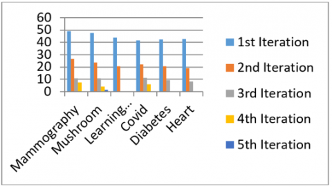
Figure 4. Reduction in boundary region size per iteration
The aforementioned algorithm was put to the test on data sets retrieved from the UCI Machine Learning Data Repository [26]. The proposed method trisects the data into three and excels at making STWD by using the Chi-square statistic as the evaluation function. As shown in Table 3, the algorithm converges into two regions-positive and negative regions-in all experiments after a fixed number of iterations.
Figure 4 depicts a graphical representation of the percentage of the boundary region size across different datasets. The figure demonstrates that with each subsequent iteration, there is a significant decrease in the size of the boundary, ultimately converging for all datasets.
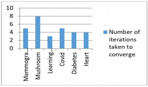
Figure 5 shows the number of iterations taken for each dataset to reach convergence to make binary decisions.
Table 3. Number of objects in the boundary region after each iteration
|
Sl. No. |
Name of The Dataset |
Total Number of Objects |
Number of Objects in The Boundary Region After Each Iteration |
The Total Number of Iterations Took to Converge |
||||
|
1st |
2nd |
3rd |
4th |
5th |
||||
|
1 |
Mammography |
961 |
472 |
257 |
106 |
73 |
- |
5 |
|
2 |
Mushroom |
8124 |
3868 |
1924 |
891 |
348 |
138 |
8 |
|
3 |
Learning disability |
378 |
166 |
78 |
- |
- |
- |
3 |
|
4 |
Covid |
1000 |
418 |
223 |
113 |
62 |
- |
5 |
|
5 |
Diabetes |
769 |
326 |
158 |
73 |
- |
- |
4 |
|
6 |
Heart |
1026 |
437 |
196 |
86 |
- |
- |
4 |
Figure 5. Number of iterations taken to converge
The use of a sequential three-way decision method in the context of granular computing was examined in this paper. To select the most optimal thresholds for performing a cosmological trisection, the Chi-square statistic was used as the objective function. Our suggested model, using Chi-square statistics, divides the boundary region into three segments at each granule level, resulting in the formation of three regions from the boundary region. At level 0, these three regions converge into the Positive and Negative regions. Concerning sequential three-way decisions, this strategy is different from earlier research. The outcomes of this research demonstrate the usefulness and efficacy of the suggested algorithm within the granularity-driven Sequential Three-Way Decision (STWD) model, particularly when complete information is not available.
The findings of this investigation have significant potential for use in various fields, enhancing decision-making by providing more knowledgeable, flexible, and statistically reliable results. Researchers are encouraged to investigate different approaches and evaluation methods, such as entropy, Fuzzy Logic-based Functions,cost-based functions, etc.to improve the method's ability to handle uncertainties and anomalies.
[1] Yao, Y. (2016). Three-way decisions and cognitive computing. Cognitive Computation, 8(4): 543-554. https://doi.org/10.1007/s12559-016-9397-5
[2] Jiang, C., Guo, D., Sun, L. (2021). Effectiveness measure for TAO model of three-way decisions with interval set. Journal of Intelligent & Fuzzy Systems, 40(6): 11071-11084. https://doi.org/10.3233/JIFS-202207
[3] Yao, Y. (2018). Three-way decision and granular computing. International Journal of Approximate Reasoning, 103: 107-123. https://doi.org/10.1016/j.ijar.2018.09.005
[4] Pedrycz, W., Chen, S.M. (Eds.). (2011). Granular computing and intelligent systems: Design with information granules of higher order and higher type. Springer Science & Business Media, Vol. 13. https://doi.org/10.1007/978- 3- 642-19820- 5
[5] Qian, J., Liu, C., Yue, X. (2019). Multigranulation sequential three-way decisions based on multiple thresholds. International Journal of Approximate Reasoning, 105: 396-416. https://doi.org/10.1016/j.ijar.2018.12.007
[6] Pauker, S.G., Kassirer, J.P. (1980). The threshold approach to clinical decision making. New England Journal of Medicine, 302(20): 1109-1117.
[7] Ma, M. (2016). Advances in three-way decisions and granular computing. Knowl.-Based Systems, 91(1): 3. http://dx.doi.org/10.1016/j.knosys.2015.10.026
[8] Merriam-Webster.com Dictionary, Merriam-Webster, https://www.merriam-webster.com/dictionary/granule.
[9] Yao, J.T., Vasilakos, A.V., Pedrycz, W. (2013). Granular computing: Perspectives and challenges. IEEE Transactions on Cybernetics, 43(6): 1977-1989. https://doi.org/10.1109/TSMCC.2012.2236648
[10] Yao, J. (2005). Information granulation and granular relationships. In 2005 IEEE International Conference on Granular Computing, 1: 326-329. https://doi.org/10.1109/GRC.2005.1547296
[11] Yao, Y. (2007). The art of granular computing. In Rough Sets and Intelligent Systems Paradigms: International Conference, RSEISP 2007, Warsaw, Poland, Springer Berlin Heidelberg. Proceedings, 1: 101-112. https://doi.org/10.1007/978-3-540-73451-2_12
[12] Yao, Y. (2013). Granular computing and sequential three-way decisions. In International conference on rough sets and knowledge technology. Berlin, Heidelberg: Springer Berlin Heidelberg, pp. 16-27. https://doi.org/10.1007/978-3-642-41299-8_3
[13] Yang, X., Li, T., Fujita, H., Liu, D., Yao, Y. (2017). A unified model of sequential three-way decisions and multilevel incremental processing. Knowledge-Based Systems, 134: 172-188. https://doi.org/10.1016/j.knosys.2017.07.031
[14] Yao, Y. (2004). A partition model of granular computing. In Transactions on Rough Sets I: James F. Peters-Andrzej Skowron, Editors-in-Chief. Berlin, Heidelberg: Springer Berlin Heidelberg, pp. 232-253. https://doi.org/10.1007/978-3-540-27794-1_11
[15] Fang, Y., Gao, C., Yao, Y. (2020). Granularity-driven sequential three-way decisions: A cost-sensitive approach to classification. Information Sciences, 507: 644-664. https://doi.org/10.1016/j.ins.2019.06.003
[16] Li, H., Zhang, L., Huang, B., Zhou, X. (2016). Sequential three-way decision and granulation for cost-sensitive face recognition. Knowledge-Based Systems, 91: 241-251. https://doi.org/10.1016/j.knosys.2015.07.040
[17] Liu, D., Liang, D., Wang, C. (2016). A novel three-way decision model based on incomplete information system. Knowledge-Based Systems, 91: 32-45. https://doi.org/10.1016/j.knosys.2015.07.036
[18] Yang, X., Li, T., Liu, D., Fujita, H. (2019). A temporal-spatial composite sequential approach of three-way granular computing. Information Sciences, 486: 171-189. https://doi.org/10.1016/j.ins.2019.02.048
[19] Yang, J., Wang, G., Zhang, Q., Chen, Y., Xu, T. (2019). Optimal granularity selection based on cost-sensitive sequential three-way decisions with rough fuzzy sets. Knowledge-Based Systems, 163: 131-144. https://doi.org/10.1016/j.knosys.2018.08.019
[20] Jia, X., Li, W., Shang, L. (2019). A multiphase cost-sensitive learning method based on the multiclass three-way decision-theoretic rough set model. Information Sciences, 485: 248-262. https://doi.org/10.1016/j.ins.2019.01.067
[21] Li, M., Wang, G. (2016). Approximate concept construction with three-way decisions and attribute reduction in incomplete contexts. Knowledge-Based Systems, 91: 165-178. https://doi.org/10.1016/j.knosys.2015.10.010
[22] Liang, D., Liu, D. (2015). Deriving three-way decisions from intuitionistic fuzzy decision-theoretic rough sets. Information Sciences, 300: 28-48. https://doi.org/10.1016/j.ins.2014.12.036
[23] Remesh, K.M., Nair, L.R. (2020). Determining optimal pair of thresholds in three-way decisions using objective functions. International Journal of Advanced Trends in Computer Science and Engineering, 9(4): July-August.
[24] Gao, C., Yao, Y. (2016). Determining thresholds in three-way decisions with Chi-square statistic. In Rough Sets: International Joint Conference, IJCRS 2016, Santiago de Chile, Proceedings. Springer International Publishing, pp. 272-281. https://doi.org/10.1007/978-3-319-47160-0_25
[25] Yao, Y. (2011). The superiority of three-way decisions in probabilistic rough set models. Information Sciences, 181(6): 1080-1096. https://doi.org/10.1016/j.ins.2010.11.019
[26] Newman, D., Hettich, S., Blake, C., Merz, C. (1998). UCI repository of machine learning databases. http://www.ics.uci.edu/~mlearn/MLRepository.html.