Fella Berrimi*![]() | Chafia Kara-Mohamed
| Chafia Kara-Mohamed![]() | Riadh Hedli
| Riadh Hedli![]() | Aboubekeur Hamdi-Cherif
| Aboubekeur Hamdi-Cherif![]()
© 2024 The authors. This article is published by IIETA and is licensed under the CC BY 4.0 license (http://creativecommons.org/licenses/by/4.0/).
OPEN ACCESS
Descriptors serve as algorithms responsible for the representation and processing of multimedia files. One of the main challenges in these algorithms involves establishing a tradeoff among conflicting performance requirements such runtime, on the one hand, and standard metrics such as accuracy, precision, recall and F-score, on the other hand. To address this challenge, a novel descriptor named Histogram of Enhanced Gradients (HEG) is introduced for noisy face recognition. The methodology behind HEG involves enhancing local gradients prior to feature extraction, corroborated by the Histogram of Oriented Gradients (HOG) descriptor and adaptive filtering. Initially, facial images are divided into blocks, and features are extracted from each block using magnitude and orientation maps to discriminate between edges, details, and flat regions. Then, these features undergo denoising with an adaptive anisotropic diffusion filter, individually customized for each of these three types. Subsequently, the enhanced histograms from the blocks are concatenated to create a comprehensive feature vector representing the original noisy face image. Finally, the HEG descriptor is integrated within a supervised machine learning scheme with a Support Vector Machine as the classifier. The proposed descriptor is evaluated not only in terms of runtime and the standard metrics cited above, but also on the basis of six other similarity metrics, across three online datasets. Experimental results, conducted under different noise levels, clearly demonstrate that the HEG descriptor outperforms nine state-of-the-art descriptors on all three datasets yielding significant enhancements in runtime efficiency, with speed improvements ranging from 1.64 to 29.56 times, and notable refinements in F-score, ranging from 1.03 to 2.39 times. These results highlight the effectiveness of the HEG descriptor in capturing facial features from multimedia noisy files.
feature extraction, histogram of oriented gradient, adaptive filter, SVM classifier, noisy face recognition
Face recognition is one of the most challenging problems in biometric systems. It has received much attention in the last two decades, or so, generating several breakthrough applications in computer vision and pattern recognition, among others [1, 2]. With the considerable increase of digital audio-visual information, it became essential to design ad hoc algorithms that allow users to define the content of the types of multimedia information - the so-called descriptors. These latter are algorithms specifically designed to possess adequate understanding of the objects within a multimedia file, facilitating easy and effective searches as well as the classification of specific requested content. In the present work, we will confine ourselves to face image recognition only.
A face recognition system involves the identification of a person by extracting distinctive features from an image of the subject's face. This process encompasses three main tasks: face detection, feature extraction, and feature classification. Face detection is the initial step, wherein the system locates and isolates the facial region in an image. Following this step, feature extraction involves capturing unique facial characteristics, such as key points or patterns. Finally, in the features classification step, the system categorizes and matches the extracted features to a pre-existing database, enabling the identification of the individual. This sequential process ensures a comprehensive and accurate face recognition outcome in a typical face recognition system.
The first step, face detection, consists in determining the location of one or more faces in the overall image [3, 4]. For detecting faces, many methods have been proposed, ranging from simple computer vision techniques, artificial neural networks to deep learning methods. One of the major contributions in face detection techniques is the algorithm of Viola and Jones [5] that works in real-time with high accuracy. It is one of the first face detection methods suitable for real-world applications that combines integral images, cascade classifiers, Haar-like features, and AdaBoost. It addresses the challenges of real-time face detection, setting a benchmark for efficiency and accuracy in the field. Some of its drawbacks include sensitivity to illumination conditions, a fixed-size window, limited resilience to pose variations, reliance on Haar-like features, and computational cost during training. Despite these limitations, the Viola and Jones algorithm has paved the way for subsequent advancements in face detection. These reasons constitute the basis for our selection in the current paper.
In the second step of face recognition, feature extraction plays a pivotal role by identifying discriminative information and well-defined features that enhance the accuracy of the subsequent classification process [6]. This step stands as one of the most explored aspects in pattern recognition, as the efficacy of classification heavily relies on the meaningfulness of data extracted from the facial image. Feature extraction methods are broadly categorized into two main approaches: feature-based and appearance-based [7]. Feature-based methods focus on geometric aspects and distinctive facial characteristics, aiming to capture specific facial details. On the other hand, appearance-based methods take a holistic approach, considering the overall facial appearance and structure.
The choice between these two categories involves a tradeoff between precision and computational efficiency. Feature-based methods may excel in capturing fine details but can be computationally intensive, while appearance-based methods provide a more holistic understanding of facial features but might overlook subtle nuances. In our approach, we opted for an appearance-based methodology due to its capacity to capture global facial patterns efficiently, aligning with our objective of achieving robust face recognition.
The feature-based approach distinguishes features such as nose, eyes, mouth using location and distance between them [8, 9]. This approach analyzes each feature as well as its spatial location with respect to other features. This information is provided to the next step, feature classification, with a standard error rate. As a result, more computations are required to locate facial features, while any error during component localization can lead to a substantial drop in accuracy. Moreover, feature-based methods suffer from many drawbacks. They tend to have limited global context thus lacking a holistic understanding of the overall appearance, making them less effective in scenarios where global context is crucial. In addition, these methods present a sensitivity to parameter settings such as the threshold for feature detection, eventually requiring further fine-tuning. Finally, these feature-based methods have limited representational power because they extract only specific points or structures. Approaches under the feature-based technique include Elastic Bunch Graph Matching (EBGM) [10], Local Binary Pattern (LBP) [11], Gradient Direction Pattern (GDP) [12], and Gabor Filter [13].
The appearance-based approach [14, 15], on the other hand, considers the facial intensity, texture color or gradient direction in order to determine the feature patterns. The feature extraction process must be efficient in terms of computing time and efficiency. The feature extraction is independent of the location of facial organs and thus makes it more popular and more effective against environmental changes. This approach has been able to manage changes in illumination conditions, shape, pose and reflectance and to sometimes handle translation and partial occlusions. Additionally, this approach is considered efficient due to its ability to retain only the significant information of images; it indeed yielded good features extraction with accurate recognition rate.
The appearance-based methods have some drawback: they suffer from computational complexity as they may have higher computational demands, especially when dealing with high-dimensional data, which can affect real-time performance. They may be less robust to local changes or occlusions since they do not focus on specific, distinctive features. The transformed features might be less interpretable, making it challenging to understand the exact characteristics contributing to the recognition. Additionally, they suffer when there is significant variability in the training data, especially when dealing with large datasets with diverse conditions. Despite these limitations, appearance-based methods are more suitable for face recognition because of their holistic character. For this reason, we chose this approach in our method. Among appearance-based approaches, we find Linear Discriminant Analysis (LDA) [16], Principal Component Analysis (PCA) [16], Locality Preserving Projections (LPP) [17] and Discrete Wavelet Transform (DWT) [18].
The third step in the face recognition process, feature classification, is devoted to establishing the class to which the unknown input query face image belongs, with the utmost accuracy and efficiency. A diverse range of classifiers comes into play, each with its unique strengths. Classifiers like Convolutional Neural Networks (CNNs) [19], Support Vector Machines (SVMs) [20], and deep learning methods [21] play a crucial role in feature classification.
CNNs are designed to automatically learn hierarchical features from input images through convolutional layers when used in feature extraction. The convolutional layers use filters to detect low-level features like edges and gradually build up to more complex features. The features extracted by the convolutional layers are then fed into fully connected layers for classification. Large datasets are typically required for training. CNNs excel in tasks like image classification, object detection, and image segmentation. They are widely used in face recognition, among others [19].
Support Vector Machines (SVMs) are very popular in face recognition and classification tasks. They discern individuals based on facial features extracted from images. Trained on facial feature datasets, SVMs establish optimal decision boundaries for effective class segregation. SVMs adapt to non-linear feature relationships using a kernel, demonstrating resilience to high-dimensional data and proficiency with modest training samples. While effective in well-structured scenarios, SVM-based face recognition systems require diverse, high-quality training data and may encounter challenges with large datasets. SVMs excel in finding optimal decision boundaries in high-dimensional feature spaces, enhancing the precision of classification. In our exploration, the choice of classifiers was guided by the complexity of facial features and the need for a robust and adaptable system. For these reasons, we have chosen SVM as our classifier [20].
Ultimately, deep learning, including deep neural networks, stand out as a versatile approach that integrates the processes of learning and feature extraction. The capacity to automatically learn hierarchical representations from data makes this approach particularly effective in handling intricate patterns and variations within facial images. The use of deep learning signifies a departure from traditional methods by allowing the system to autonomously discern relevant features for classification [21].
In summary, a standard face recognition system initiates with face detection, identifying faces, followed by feature extraction to generate a distinctive representation for each face. The concluding step encompasses the comparison of these features with a database for recognition and classification. The integration of these three steps guarantees precise and efficient face recognition across diverse applications such as surveillance, security, and authentication systems.
In this paper, we address the issue of feature extraction of noisy face images. It is widely admitted that face recognition systems always suffer from natural degradations such as noise. Therefore, recognizing noisy images is a complex task for machines. As a result, efficient descriptors are needed.
We propose the so-called Histogram of Enhanced Gradients (HEG) as a new fast descriptor, whose main function is to ensure a tradeoff between recognition performance like runtime and standard metrics, such as precision, accuracy, recall and F-score, while addressing some issues faced by the Histogram of Oriented Gradients (HOG) such as the block size used for dividing images [22].
We attempt to improve HOG because it is one of the most powerful descriptors, so far. Its power comes from the fact that it uses magnitude as well as angle of gradient to compute the features. However, one of the drawbacks of the HOG descriptor is that its performance in both the feature extraction step and the classification step is highly impacted by noise. In order to improve the HOG descriptor, we apply a method based on coupling anisotropic diffusion and shock filter for different gradient values on each block of face image. The extracted features are the distribution of oriented smoothed gradients of face image [23].
The local object appearance is described by the distribution of intensity gradient and its direction. As a result, three types of areas are identified: edges (fine features) correspond to large gradient values, details (small features) correspond to medium gradient values, and the flat areas (large features) correspond to smaller gradient values. The separation of different regions in each block of face image requires an adaptive denoising method to be performed according to the region type. Consequently, the HEG descriptor is found to be more powerful than HOG.
This paper seeks to achieve the following contributions:
(1) Enhance the HOG descriptor by adding an adaptive anisotropic diffusion filter to recover degraded features. Use an enhanced gradient map and compute the orientation map of each block in the face image, thus generating a new compact feature vector of the noisy face image for fast classification.
(2) Include the denoising task within the feature extraction step to enhance the different objects and extract more discriminative features so that the novel descriptor can efficiently filter noisy features.
(3) Use a thresholding algorithm to process 3 types of features for each block of image.
(4) Use the HEG descriptor in a standard supervised machine scheme with SVM as the classifier with a linear kernel to undertake a comparison between the proposed descriptor and nine well-known descriptors, namely Histogram of Oriented Gradients (HOG) [22], Local Ternary Patterns (LTP) [24], Local Gradient Code (LGC) [25], Local Phase Quantization (LPQ) [26], Local Directional Number (LDN) [27], Local Gradient Pattern (LGP) [28], Local Binary Pattern (LBP) [11], Principal Component Analysis (PCA) [16], and Gabor Filter [13].
(5) Use three datasets such as Extended CK+ color dataset [29] as well as gray scale datasets like Extended Yale B [30] and ORL [31], for experiments.
The rest of this paper is organized as follows. Section 2 describes related works. Section 3 describes the proposed approach. The experimental results as well as discussions are presented in Section 4. Finally, Section 5 concludes the paper and proposes some potential future research avenues.
Before delving into specific methods, it is essential to establish a broader context surrounding the intricate challenges faced by facial feature extraction. This step plays a pivotal role in face recognition systems, involving the identification and extraction of distinctive facial characteristics for subsequent analysis. This process is critical for the accurate classification of facial images and plays a central role in the overall effectiveness of face recognition. In this section, we elucidate key contributions in the field, outlining notable descriptors that hold widespread significance. The subsequent descriptions report the most popular descriptors.
The Local Binary Pattern (LBP) [11] is one of the most popular local region-based feature descriptors, adopted for both objects and human face. This method consists in comparing the pixel gray level with those of its neighbors. It assigns a binary code to a pixel according to its neighborhood. This method recognizes certain local binary patterns considered as uniform. However, the LBP method has the drawback of losing global spatial information. To address this issue, many variants of LBP have been developed, with various degrees of success for many tasks: LBP Variance (LBPV) [32] and Local Gabor Binary Pattern Histogram Sequence (LGBPHS) [33].
Additionally, the Local Gradient Code (LGC) [25], a variant of the LBP, describes the gradient of the horizontal, vertical, and diagonal details of the facial image. On the other hand, the Local Ternary Patterns (LTP) [24] stands as another generalization of the LBP. It is reported to be more discriminant and less sensitive to noise in uniform regions. LTP relies on two main components: the integration of Principal Component Analysis (PCA) for feature extraction, on the one hand, and additional sources, namely Gabor wavelets and LBP, on the other hand. It was found that this combination gave better accuracy [24]. With all these offshoots, LBP gained a good ranking among the discrimination techniques for face extraction.
Local Phase Quantization (LPQ) [26] is another well-known feature-based technique. It builds on the blur invariance property of short time Fourier transform to extract the image features. This technique ends up with more accurate and stable classification results. However, one limitation of LPQ is its slowness in some cases, especially when the number of features is high.
The LDN method [27] compactly converts the directional information of face's textures, in an attempt to produce a more discriminative code than other descriptors. The structure is evaluated for each micro-pattern using a compass mask that extracts directional information. The encoding of such information is done using the prominent direction indices (directional numbers) and sign. This latter allows the distinction between similar structural patterns with different intensity transitions. The face is divided into several regions. These features are then concatenated into a feature vector and tested with different masks.
The Scale Invariant Feature Transform (SIFT) [34] performs best in the context of matching and recognition, due to its invariance to scaling and rotations. Several attempts to improve the SIFT descriptor have been proposed in the literature, such as PCA-SIFT [35].
Another feature extraction method is proposed using wavelet packet frame decomposition and Gaussian-mixture-based classifier to assign each pixel to the class [36]. Each subnet of the classifier is modeled by a Gaussian mixture model and each texture image is assigned to the class to which the pixels of the image belong mostly.
The Weber Local Descriptor (WLD) [37] is based on the fundamental concept that human perception of patterns is intricately tied to the change of a stimulus. This idea holds particular significance in the context of the WLD method as it aligns with the manner in which distinctive facial features are perceived and processed. Human visual perception is highly attuned to changes and variations in patterns, and the WLD method enhances this cognitive aspect to capture meaningful information from facial images.
In the Local Directional Pattern (LDP) method [38], the feature is obtained through the evaluation of the edge response values for each pixel position in all eight directions. A code is then generated from the relative strength magnitude. Each bit of code sequence gains robustness in noisy situations since it is based on the local neighborhood. An LDP code, which is rotation invariant, is introduced which uses the direction of the most prominent edge response. Finally, an image description is obtained for the image by the accumulation of the occurrence of LDP feature over the whole input image. Experimental results show that LDP gives better results than Gabor-wavelet and LBP.
Some statistical methods that are insensitive to blur, have been used for feature extraction. However, these methods are not rotation invariant, like Gabor Filter [13] and wavelet transform [18]. Other discriminative techniques were also explored in feature classification such as Local Gradient Pattern (LGP) [28], Gradient Direction Pattern (GDP) [12], Eigenfaces based PCA [16], Linear Discriminant Analysis (LDA) [16], and Histogram of Orientation Gradient (HOG) [22].
3.1 Motivation
In this section, providing insights into the primary motivations, we introduce the innovative HEG descriptor. The initial phase of the conventional HOG involves calculating the gradient magnitude at each pixel, followed by dividing the face image into for n×m blocks. Each block is then represented by a histogram capturing the local distribution of orientations and gradient amplitudes. However, as we provide details about the HEG descriptor, we address certain limitations inherent in the traditional HOG approach.
One notable limitation we address is related to the block size in HOG. While the optimal block size for pedestrian detection has been identified as for 3×3 blocks [22], our experimentation reveals improved classification performance with larger for 8×8 blocks. This adjustment enhances the block area by a factor of 7, resulting in a reduction in runtime, logically aligning with the need for efficiency in facial feature extraction. Additionally, another limitation of the HOG descriptor that we address is its sensitivity to noise. The HEG descriptor incorporates an adaptive anisotropic diffusion step, refining the features extracted by HOG based on the type of pixel, namely edge, detail, or flat region. This ad hoc enhancement process mitigates the impact of noise on feature extraction, ensuring that the HEG descriptor maintains robust performance in the presence of challenging conditions.
Hence, the HEG descriptor, while enhancing runtime efficiency through optimized block sizes, improves the robustness of feature extraction by reducing sensitivity to noise. By adapting the approach to tackle these specific limitations, the HEG descriptor emerges as a refined and more effective alternative to traditional HOG in facial feature extraction.
3.2 Overall architecture
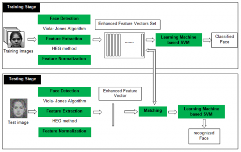
The HEG descriptor is used within a broader supervised learning scheme, comprising the two main classical phases of training and classification. Figure 1 shows the overall architecture where the HEG descriptor is used.
Figure 1. Diagram of proposed framework
3.2.1 Training phase
In any supervised learning scheme, the training phase comes first. Here, after detecting the image, using the Viola & Jones algorithm [5], the HEG descriptor is applied for the whole face in order to create its enhanced feature vector through extraction followed by normalization. Then, the image is saved in the database with its corresponding class, using SVM classifier [20].
3.2.2 Classification phase
In the classification step, the unknown query image is represented by a vector by applying HEG descriptor. The enhanced feature vector is normalized as in the training phase, and then fed into the SVM classifier to determine the best match between the query and previous training images. The details of the HEG descriptor operation are given in the sub-section below.
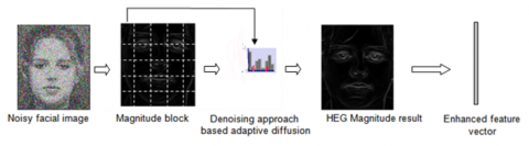
3.3 HEG steps
HEG obeys the following steps (see Figure 2):
Step 1. Decompose the whole input noisy image into n×m non-overlapping blocks. Then, calculate the gradient of each pixel in the block. The gradient magnitude at each pixel of a block is used for feature separation as it discriminates between the different types of features such as edges, details, and homogeneous regions. The norm of the gradient in a pixel is useful information because the magnitude is large around edges due to abrupt changes in intensity which keeps more information about the object shape than flat regions.
As a result, these regions have to be processed differently to obtain good classification. For doing so, a block is subdivided into three types of regions using a threshold segmentation method based on gray level gradient histogram that defines two thresholds T1 and T2, proper to each block [39]. Each block is therefore segmented into three regions: large gradients (greater than T2) describing boundaries of different objects, while medium gradients (between T1 and T2) determining textures and details, finally, small gradients (lower than T1) representing flat regions of the image.
Step 2. Represent each block by a histogram with 3 gradient bins, each one determining the interval that can describe edges, details or flat regions. In this step, the enhanced features are provided by HEG that denoises each block according to the type of features. An adaptive diffusion denoising step is initiated to properly recover each region in a block in accordance with its type. For edges, a shock-type backward diffusion is applied in the gradient direction. A soft backward diffusion is performed to enhance image details preserving a natural transition. Moreover, an isotropic diffusion is used to smooth homogeneous areas simultaneously. Therefore, each pixel is represented with enhanced intensity in the respective direction.
Step 3. Represent features on magnitudes and orientation maps in polar coordinates system (G, θ). The enhanced magnitude (G) values of each block in the histogram are the votes and the orientation maps values (θ) are represented with 9 orientation bins. The magnitude G and angle θ, are given by:
$G=\sqrt{G_x^2+G_y^2}$ (1)
$\theta=\tan ^{-1}\left(\frac{G_y}{G_x}\right)$ (2)
where, Gx and Gy represent gradients in horizontal and vertical directions respectively.
Step 4. Normalize all enhanced histograms blocks to finally obtain the feature vectors. Each face image in the training set is saved as a features vector that will be used in the classification phase. The orientation of a pixel in each block is placed into one of 9 orientation bins weighted by its magnitude to create a weighted histogram for each block. Concatenating all normalized histograms produces the extracted feature vector which is used to prepare the input noisy face image for the SVM classifier. Finally, the HEG descriptor concatenates all normalized histograms.
Note that, in our case, noise doesn't affect the performance of face recognition since the denoising is performed with an adaptive diffusion filter, based on partial differential equations, which is an efficient tool of enhancement and restoration of edge and details information.
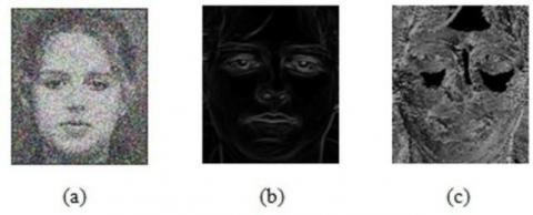
For illustration purposes of the HEG descriptor image enhancement, Figure 3 shows the original image and the corresponding HEG results, as outputs produced by the descriptor. Figure 3(a) shows the noisy input image to be processed, Figure 3(b) shows the magnitude gradient result and Figure 3(c) shows the orientation map result. It is to be noted that the enhancements are destined to the computer program and not to be used for immediate normal human visual purposes.
Figure 2. Main steps of HEG descriptor
Figure 3. (a) Noisy image (b) HEG magnitude result (c) HEG orientation result
All subsequent experiments were carried out on a laptop with Intel Core™ i5-6200U CPU 2.40GHz, 8 GB RAM, using Windows™ 10, 64-bit system. For implementation, we used Python and the sklearn library (https://scikit-learn.org/stable/) to facilitate coding of machine learning.
4.1 Chosen competitors and datasets
A comparative assessment is undertaken between the HEG descriptor and nine other descriptors using three different datasets in grayscale as well as in color. The main experiment is the same for all datasets, namely to classify a noisy face image with various descriptors using the SVM classifier. This latter is used because it was proved to produce the best classification in the shortest time.
(1) The chosen competitors are: LTP [24], LGC [25], LPQ [26], LDN [27], LGP [28], LBP [11], PCA [16], HOG [22] and Gabor Filter [13].
(2) The datasets used are: Extended Cohn-Kanade (CK+) dataset [29], Extended Yale B dataset [30], and ORL dataset [31].
4.2 Evaluation metrics
To compare descriptors, we rely on the usual standard metrics of image recognition. Our goal is to find a tradeoff between these conflictual metrics.
4.2.1 Standard metrics
All descriptors are tested using the well-known standard metrics, namely accuracy, precision, recall and F-score, widely used in many areas. We added runtime, i.e., the time needed to accomplish the final classification phase.
4.2.2 Similarity metrics
In addition, we also rely on similarity metrics [40, 41] such as: Mean Square Error (MSE), Peak Signal-to-Noise Ratio (PSNR), Structural Similarity Index (SSIM), Features Similarity Index Matrix (FSIM), Three-component SSIM (3-SSIM) and Normalized Absolute Error (NAE).
4.2.3 HEG descriptor gain
As for HEG descriptor gain, we have to distinguish between two cases:
(1) Metrics to be maximized, i.e., all standard metrics above in addition to SSIM, FSIM, PNSR. In this case, the gain is defined as the ratio of the HEG descriptor metric value divided by the corresponding competitor's metric value. For example, for ORL dataset, F-score gain of HEG w.r.t. LTP=92.25/41.77=2.21, meaning that HEG descriptor F-score is 2.21 times better than that of LTP.
(2) Metrics to be minimized, i.e., runtime, MSE, and NAE. The HEG descriptor gain is now defined as the ratio of the competitor's metric value divided by HEG descriptor metric value. For example, runtime gain of HEG w.r.t. PCA, for ORL dataset is 18.76, meaning that HEG descriptor is 18.76 faster than PCA. Note that the gain has to be strictly greater than unity.
4.3 Experiments on ORL dataset
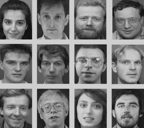
ORL dataset [31] is a publicly available and widely adopted benchmark for the evaluation of face recognition. This dataset contains 400 images from 40 distinct subjects. For some subjects, the images were taken at different times, varying the lighting, facial expressions (open/closed eyes, smiling / not smiling) and facial details (glasses/no glasses). All images are taken against a dark homogeneous background with subjects in an upright, frontal position (with tolerance for some side movement). The size of each image is 92×112 pixels, with 256 grey levels per pixel. Figure 4 shows sample images of the ORL dataset.
Figure 4. Samples of ORL dataset
4.3.1 Convenient size of blocks
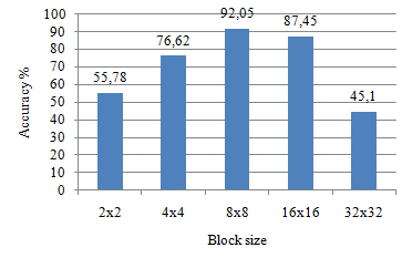
We carried out different experiments on ORL dataset to determine the convenient size of blocks that contain various regions. This preliminary experiment allowed us to correctly separate these regions into blocks, so that we can perform the enhancement processing efficiently. We further studied the impact of block size on classification accuracy. The HEG descriptor was applied to blocks of different sizes: 2×2, 4×4, 8×8, 16×16 and 32×32. The results are reported on Figure 5; clearly showing that a block of size 8×8 gives the best accuracy for an image of 92×112 with HEG descriptor. Note that the small block dimension ignored the edges and fine details.
Figure 5. HEG accuracy for different block sizes with ORL dataset
4.3.2 Noisy inputs
We then added a white additive Gaussian noise with different values of variance (0, 0.2, 0.4, 0.8, 1.2). This experiment was done in order to check the HEG stability in a noisy environment and to evaluate the performance of the denoising process in each block. After the denoising process, we estimated the quality of recovered image using 3-SSIM and FSIM metrics, measured as the average of 3-SSIM and FSSIM values of blocks on image. Table 1 illustrates the results. Note that the first value shows that the image is not corrupted by noise; it is considered as a reference image.
From Table 1, we can see that the metrics 3-SSIM and FSSIM give consistent results, because the denoising process is performed according to the type of each region in the block. The quality of the image, as measured by FSSIM, is between 0.991 and 0.978, and, with 3-SSIM, between 0.990 and 0.977 with noise variance less than unity. The results are acceptable for noise variance up to 1.2, where HEG descriptor achieves the best contribution.
Table 1. FSSIM and 3-SSIM measures before and after applying HEG on ORL dataset
|
|
Before HEG |
After HEG |
||
|
variance |
3-SSIM |
FSSIM |
3-SSIM |
FSSIM |
|
0 |
0.992 |
0.994 |
0.994 |
0.995 |
|
0.2 |
0.985 |
0.987 |
0.990 |
0.991 |
|
0.4 |
0.978 |
0.981 |
0.984 |
0.987 |
|
0.6 |
0.972 |
0.976 |
0.978 |
0.983 |
|
0.8 |
0.967 |
0.968 |
0.977 |
0.978 |
|
1.2 |
0.928 |
0.915 |
0.942 |
0.948 |
4.3.3 Descriptors standard metrics on ORL dataset
We evaluated the performance of our model on ORL dataset using an image corrupted by white additive Gaussian noise with variance 0.8 as test image, and the remaining images used as training set for the SVM classifier. Table 2 and Figure 6 show the performance comparison results of different descriptors (LTP, LGC, LPQ, LDN, LGP, LBP, PCA, HOG, Gabor Filter) on ORL database.
Table 2 shows the accuracy, F-score of related descriptors, HEG accuracy gain and HEG F-score gain on the ORL dataset. It is noted that HEG attains high accuracy with 92.05% and high F-score with 92.25% immediately followed by HOG descriptor. This remains to the acquisition conditions of images on ORL database. For easy readability, in Table 2 and in all subsequent tables, the best results are indicated in bold.
Table 2. Descriptors standard metrics and corresponding HEG descriptor gains (ORL dataset)
|
Descriptor |
Accuracy |
F-Score |
Accuracy Gain |
F1-Score Gain |
|
LTP |
40.82 |
41.77 |
2.26 |
2.21 |
|
LGC |
78.85 |
76.38 |
1.17 |
1.21 |
|
LPQ |
72.25 |
70.04 |
1.27 |
1.32 |
|
LDN |
65.54 |
48.34 |
1.40 |
1.91 |
|
LGP |
80.45 |
78.98 |
1.14 |
1.17 |
|
LBP |
64.45 |
63.24 |
1.43 |
1.46 |
|
PCA |
39.22 |
40.17 |
2.35 |
2.30 |
|
HOG |
89.07 |
88.1 |
1.03 |
1.05 |
|
Gabor Filter |
88.85 |
89.19 |
1.04 |
1.03 |
|
HEG |
92.05 |
92.25 |
1.00 |
1.00 |
Figure 6. HEG descriptor gain on standard metrics (ORL dataset)
Figure 6 shows the HEG gains in terms of accuracy and F-score, in comparison with all competitors. The HEG descriptor improves the accuracy by a factor ranging from 1.03 (w.r.t. HOG) and 2.35 (w.r.t. PCA). This means that the HEG descriptor improves HOG accuracy by 3% and PCA accuracy by 135%. Additionally, it improves the F-score by a factor from 1.03 (Gabor Filter) and 2.30 (PCA): the improvement in F-score is 3% over Gabor Filter and 130% over PCA.
4.3.4 Descriptors similarity metrics on ORL dataset
To measure the classification rate, we compute the similarity between the query face and each training face in the class using similarity metrics: MSE, PSNR, SSIM, FSSIM and NAE. Table 3 reports the similarity metrics values of all descriptors. Figure 7 shows the PSNR, SSIM and FSSIM gains of all descriptors. We can easily notice that the HEG descriptor outperforms all competitors: it attains the highest FSSIM and SSIM of 0.98 and 0.97. On the other hand, HEG also achieves the lowest MSE (4.29), and the lowest NAE (0.08).
Table 3. Descriptors similarity metrics (ORL dataset)
|
Descriptor |
MSE |
PSNR |
SSIM |
FSSIM |
NAE |
|
LTP |
11.68 |
37.45 |
0.795 |
0.712 |
0.65 |
|
LGC |
9.04 |
38.56 |
0.875 |
0.810 |
0.25 |
|
LPQ |
10.00 |
38.13 |
0.840 |
0.790 |
0.32 |
|
LDN |
10.98 |
37.72 |
0.810 |
0.742 |
0.34 |
|
LGP |
6.89 |
39.74 |
0.895 |
0.855 |
0.20 |
|
LBP |
11.25 |
37.61 |
0.802 |
0.705 |
0.60 |
|
PCA |
12.98 |
36.99 |
0.745 |
0.697 |
0,61 |
|
HOG |
5.81 |
40.48 |
0.952 |
0.945 |
0.088 |
|
Gabor Filter |
6.54 |
39.97 |
0.938 |
0.904 |
0.11 |
|
HEG |
4.29 |
41.80 |
0.974 |
0.978 |
0.079 |
Figure 7. HEG descriptor gain on 3 similarity metrics (ORL dataset)
The proposed method demonstrates a stronger similarity with the ORL dataset, where HEG achieves the highest FSSIM score across all testing images in our experiments. These results substantiate the capability of HEG in recognizing a person's face captured under noise. This effectiveness can be attributed to the denoising filter's performance, which is applied in each block based on the specific characteristics of each feature.
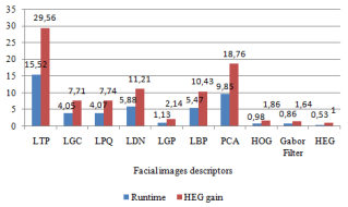
4.3.5 Descriptors runtime on ORL dataset
Table 4 and the corresponding Figure 8 illustrate the runtime for all descriptors under study, for the ORL dataset. The last column on the right in Table 4 shows the runtime gain of the HEG. For instance, it is shown that the HEG descriptor achieves the lowest runtime 0.53s, improving its immediate competitor runtime (Gabor Filter) by 64%. It further improves HOG descriptor runtime by 86% and is approximately 29 times faster than the farthest competitor (LTP). We notice that the runtime significantly decreases with the feature extraction method.
Table 4. Descriptors runtime and HEG descriptor time gain (ORL dataset)
|
Descriptor |
Runtime (s) |
HEG Gain |
|
LTP |
15.52 |
29.56 |
|
LGC |
4.05 |
7.71 |
|
LPQ |
4.07 |
7.74 |
|
LDN |
5.88 |
11.21 |
|
LGP |
1.13 |
2.14 |
|
LBP |
5.47 |
10.43 |
|
PCA |
9.85 |
18.76 |
|
HOG |
0.98 |
1.86 |
|
Gabor Filter |
0.86 |
1.64 |
|
HEG |
0.53 |
1.00 |
Figure 8. Descriptors runtime and HEG descriptor time gain (ORL dataset)
4.4 Experiments on CK+ dataset
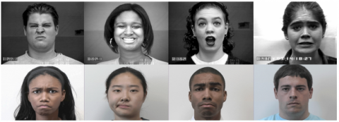
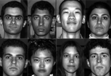
The Extended Cohn-Kanade (CK+) dataset contains 593 video sequences from a total of 123 different subjects, ranging from 18 to 50 years of age with a variety of genders and heritage [33]. Each video shows a facial shift from the neutral expression to a targeted peak expression, recorded at 30 frames per second with a resolution of either 640×490 or 640×480 pixels. Out of these videos, 327 are labeled with one of seven expression classes: anger, contempt, disgust, fear, happiness, sadness, and surprise. These images are resized to 92×128 pixels with grayscale representation that helps in simplifying computational requirements. Figure 9 shows samples of CK+ dataset.
Figure 9. Samples of CK + dataset
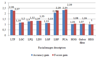
4.4.1 Descriptors standard metrics on CK+ dataset
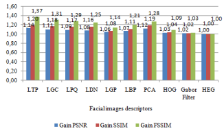
We evaluated the performance of all descriptors in terms of standard metrics on CK+ dataset. We used different face images corrupted by white additive Gaussian noise of variance 0.8. As shown in Table 5 and Figure 10, the HEG descriptor achieves both the highest accuracy (91.63%) and the highest F-score (91.78%). More precisely, the HEG descriptor improves both the accuracy and the F-sore of its immediate competitor (HOG) by 5% and 8%, respectively. On the other extreme, the HEG descriptor improves the accuracy of LTP by 136% and the F-score of PCA by 139%.
Table 5. Descriptors standard metrics and corresponding HEG descriptor gains (CK+ dataset)
|
Descriptors |
Accuracy |
F-Score |
Accuracy Gain |
F-Score Gain |
|
LTP |
38.85 |
40.48 |
2.36 |
2.27 |
|
LGC |
77.37 |
76.3 |
1.18 |
1.20 |
|
LPQ |
70.42 |
69.57 |
1.30 |
1.32 |
|
LDN |
68.41 |
68.12 |
1.34 |
1.35 |
|
LGP |
80.95 |
81.02 |
1.13 |
1.13 |
|
LBP |
43.91 |
40.15 |
2.09 |
2.29 |
|
PCA |
39.10 |
38.39 |
2.34 |
2.39 |
|
HOG |
86.77 |
85.12 |
1.05 |
1.08 |
|
Gabor Filter |
85.25 |
84.28 |
1.07 |
1.09 |
|
HEG |
91.63 |
91.78 |
1.00 |
1.00 |
Based on these results, it can be observed that HEG, which is based on adaptive diffusion of gradients, outperforms the related descriptors. This can be attributed to the effective techniques employed for both feature segmentation using gradient maps and feature restoration through anisotropic diffusion.
As a result, HEG demonstrates promising performance in handling degraded facial images when compared to other conventional descriptors on the CK+ database.
Figure 10. HEG descriptor gain on standard metrics (CK+ dataset)
4.4.2 Descriptors similarity metrics on CK+ dataset
We further evaluated the similarity metrics, described above, on CK+ dataset. According to Table 6 and Figure 11, it is noted that HEG descriptor achieves the highest SSIM similarity measure (0.964), the highest FSSIM (0.978), the highest PSNR (41.30). On the other hand, HEG also achieves the lowest MSE (5.00), and the lowest NAE (0.081). The classification is carried out at feature level where no information is lost.
As far as similarity metrics are concerned the HEG descriptor is proved to be an efficient descriptor for face recognition on CK+ dataset. It is noted that the Gabor Filter results are close to standard HOGs results. This is so, because the Gabor Filter applies a wavelets-based filter prior to feature extraction.
Table 6. Descriptors similarity metrics (CK+ dataset)
|
Descriptor |
MSE |
PSNR |
SSIM |
FSSIM |
NAE |
|
LTP |
18.92 |
35.36 |
0.789 |
0.704 |
0.68 |
|
LGC |
15.95 |
36.10 |
0.845 |
0.781 |
0.34 |
|
LPQ |
16.45 |
35.96 |
0.824 |
0.765 |
0.45 |
|
LDN |
17.25 |
35.76 |
0.818 |
0.742 |
0.48 |
|
LGP |
11.36 |
37.57 |
0.876 |
0.805 |
0.19 |
|
LBP |
17.89 |
35.60 |
0.801 |
0.719 |
0.62 |
|
PCA |
18.68 |
35.41 |
0.792 |
0.711 |
0.64 |
|
HOG |
6.90 |
39.73 |
0.935 |
0.945 |
0.099 |
|
Gabor Filter |
7.69 |
39.26 |
0.918 |
0.897 |
0.108 |
|
HEG |
5.00 |
41.30 |
0.964 |
0.978 |
0.081 |
Figure 11. HEG descriptor gain on 3 similarity metrics (CK+ dataset)
4.4.3 Descriptors runtime on CK+ dataset
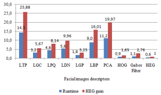
We finally evaluated the runtime of the HEG descriptor on CK+ dataset. Figure 12 shows the runtime of all descriptors. The shortest runtime is obtained by HEG (0.561s), and is proved to be 65% faster than its immediate competitor (HOG, with runtime of 0.925s). As seen in Table 7, HEG is approximately 25.9 times faster than the slowest descriptor (LTP, with a runtime of 14.52s).
Figure 12. Descriptors runtime and HEG descriptor time gain (CK+ dataset)
Table 7. Descriptors runtime and HEG descriptor time gain (CK+ dataset)
|
Descriptor |
Runtime (s) |
HEG Gain |
|
LTP |
14.52 |
25.88 |
|
LGC |
3.182 |
5.67 |
|
LPQ |
4.565 |
8.14 |
|
LDN |
5.588 |
9.96 |
|
LGP |
1.825 |
3.25 |
|
LBP |
8.984 |
16.01 |
|
PCA |
11.205 |
19.97 |
|
HOG |
0.925 |
1.65 |
|
Gabor Filter |
1.147 |
2.76 |
|
HEG |
0.561 |
1.00 |
4.5 Experiments on Extended Yale B dataset
The Extended Yale B dataset contains 2414 frontal-face images with size 192×168 over 38 subjects and about 64 images per subject [34]. The images were captured under different lighting conditions and various facial expressions. In our work, we only considered the frontal images. Figure 13 presents samples of this dataset.
Figure 13. Samples of Extended Yale B dataset
4.5.1 Descriptors standard metrics on Extended Yale B dataset
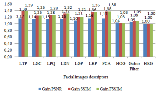
We evaluated the performance of all descriptors on Extended Yale B dataset, with different face images corrupted by white additive Gaussian noise of variance 0.8. Table 8 and Figure 14 report the results. Based on the values displayed, we can see that the HEG descriptor gives the highest accuracy (92.82%) and the highest F-score (92.24%). We clearly observe that the HEG descriptor improves the F-score of Gabor filter and HOG by 8% and 9%, respectively. Besides, the HEG descriptor F-score gain is 2.39 better than LTP, i.e., it improves LTP F-score by 139% on Extended Yale B images.
As for the accuracy, the HEG descriptor improves its immediate competitor (Gabor Filter) by 7% and its farthest one (LTP) by 133%.
Table 8. Descriptors standard metrics and corresponding HEG descriptor gains (Extended Yale B dataset)
|
Descriptor |
Accuracy |
F-Score |
Accuracy Gain |
F-Score Gain |
|
LTP |
39.85 |
38.58 |
2.33 |
2.39 |
|
LGC |
64.82 |
63.77 |
1.43 |
1.44 |
|
LPQ |
65.95 |
64.96 |
1.41 |
1.42 |
|
LDN |
66.43 |
66.31 |
1.40 |
1.39 |
|
LGP |
75.31 |
75.12 |
1.23 |
1.22 |
|
LBP |
65.87 |
64.98 |
1.41 |
1.42 |
|
PCA |
40.15 |
40.55 |
2.31 |
2.27 |
|
HOG |
85.77 |
84.61 |
1.08 |
1.09 |
|
Gabor Filter |
86.42 |
85.16 |
1.07 |
1.08 |
|
HEG |
92.82 |
92.24 |
1.00 |
1.00 |
Figure 14. HEG descriptor gain on standard metrics (Extended Yale B dataset)
These results enhance the feature segmentation method employed in our study, leading to improved classification performance by utilizing the enhanced gradient map generated by HEG. Consequently, the proposed feature extraction operator demonstrates increased efficiency.
4.5.2 Descriptors similarity metrics on Extended Yale B dataset
Figure 15. HEG descriptor gain on 3 similarity metrics (Extended Yale B dataset)
We used similarity metrics to evaluate the descriptors on the Extended Yale B dataset. Table 9 and Figure 15 display the results. Note that HEG has the best values across all similarity metrics on Extended Yale B dataset with the smallest MSE (5.08) and NAE (0.08) The HEG descriptor attains the highest PSNR, SSIM and FSSIM with 41.09, 0.95 and 0.98, respectively. It is clearly a tangible achievement for noisy face recognition in a dataset of this size and complexity. The HEG descriptor is immediately followed by Gabor Filter, for all similarity metrics. The minimum improvement is 2% for all of SSIM FSSIM and PNSR. The maximum improvement is 20% for SSIM, 14% for FSSIM and 37% for PNSR, w.r.t. LTP.
Table 9. Descriptors similarity metrics (Extended Yale B dataset)
|
Descriptor |
MSE |
PSNR |
SSIM |
FSSIM |
NAE |
|
LTP |
15.84 |
36.13 |
0.789 |
0.712 |
0.69 |
|
LGC |
12.78 |
37.06 |
0.804 |
0.745 |
0.35 |
|
LPQ |
11.32 |
37.59 |
0.810 |
0.761 |
0.46 |
|
LDN |
10.46 |
37.93 |
0.815 |
0.782 |
0.48 |
|
LGP |
8.28 |
38.94 |
0.880 |
0.855 |
0.22 |
|
LBP |
9.34 |
38.42 |
0.852 |
0.810 |
0.45 |
|
PCA |
14.26 |
36.58 |
0.792 |
0.765 |
0,65 |
|
HOG |
6.91 |
39.73 |
0.910 |
0.894 |
0.12 |
|
Gabor Filter |
5.99 |
40.35 |
0.928 |
0.945 |
0.115 |
|
HEG |
5.08 |
41.09 |
0.946 |
0.978 |
0.079 |
4.5.3 Descriptors runtime on Extended Yale B dataset
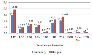
We compared the runtime of all descriptors on the Extended Yale B dataset. Table 10 and the corresponding Figure 16 show that the HEG descriptor has the shortest time as compared with other descriptors. It achieves 0.76 seconds, improving its immediate competitor runtime (Gabor Filter) by approximately 28%. It further improves HOG descriptor by 33% and is approximately 18 times faster than its farthest competitor (LTP).
Figure 16. Descriptors runtime and HEG descriptor time gain (Extended Yale B dataset)
Table 10. Descriptors runtime and HEG descriptor time gain (Extended Yale B dataset)
|
Descriptor |
Run Time (s) |
HEG Gain |
|
LTP |
14,75 |
19,28 |
|
LGC |
3,815 |
4,98 |
|
LPQ |
5,825 |
7,61 |
|
LDN |
5,143 |
6,72 |
|
LGP |
1,258 |
1,64 |
|
LBP |
8,654 |
11,31 |
|
PCA |
10,451 |
13,66 |
|
HOG |
1,018 |
1,33 |
|
Gabor Filter |
0,984 |
1,28 |
|
HEG |
0,765 |
1,00 |
The comparison of descriptors runtime demonstrates the effectiveness of the HEG descriptor in performing fast classification on Extended Yale B dataset. We note that all descriptors consume much longer time than the HEG descriptor.
4.6 Discussion
In this study, we aimed to develop a model for accurate classification of face images captured under noisy conditions. We used SVM as the machine learning algorithm and implemented a descriptor based on HOG with adaptive diffusion (HEG) to improve feature extraction and recognition. Key lessons learned from this work include:
(1) Face recognition systems often encounter degradations like noise due to the inherent difficulties in capturing perfect images. Consequently, machine-based recognition of these images becomes a complex task. To improve accuracy, efficient descriptors are essential for classifying noisy face images. In this work, we implemented a descriptor based on HOG with adaptive diffusion, creating an enhanced feature vector that yielded the best classification results.
(2) The study explored the impact of block size on feature recovery and classification. By considering various block structures, the features were effectively recovered, resulting in efficient classification.
(3) The proposed model identified noisy face images through experimental testing using different levels of variance in noise. The quality of denoised images after applying HEG was assessed using the 3-SSIM evaluation metric, which considers three regions (edges, details, and homogeneous regions). The results indicated that HEG effectively described corrupted faces, leading to superior classification performance.
(4) The proposed approach was compared to nine standard descriptors. The performance evaluation of the proposed descriptor demonstrated significant improvements in accuracy, F1-score, MSE, NAE, PSNR, SSIM and FSSIM across three face databases. Notably, the HEG model outperformed other descriptors in both color and grayscale spaces. Additionally, HEG exhibited increased efficiency and significantly reduced execution time.
Based on the experiments conducted, HEG outperforms other operators in terms of feature extraction and noisy face recognition.
In this article, we presented the HEG descriptor, designed and evaluated for the efficient and rapid recognition of noisy facial images. The methodology is based on the extraction of enhanced features through a two-step process. Initially, the HOG method is utilized to capture both orientation and intensity information across facial regions. The selection of the HOG descriptor is based on its capability in capturing detailed gradient information, effectively emphasizing facial features.
Subsequently, an adaptive anisotropic diffusion is applied, fine-tuning the enhancement, on the basis of pixel characteristics: edge, detail, or flat region. This differentiation is achieved through a thresholding algorithm based on magnitude gradient and orientation maps. The subsequent adaptive anisotropic diffusion refines this information, customizing the enhancement process to the specific characteristics of different facial regions. This dual-stage approach allows the HEG descriptor to efficiently recognize noisy facial features. As shown in the experiments, the integration of these methods significantly enhances the recognition process.
Experimental validation on diverse datasets, including color (Extended CK+) and grayscale (ORL, Extended Yale B datasets), involved a comprehensive comparison with nine state-of-the-art descriptors for facial feature extraction and classification. The results, obtained under varying levels of noise variance, unequivocally demonstrated the superiority of the HEG descriptor. It not only gave the fastest runtime but also outperformed all competitors across multiple metrics such as accuracy, F-score, MSE, NAE, PSNR, SSIM, and FSSIM, in both color and grayscale contexts.
Looking ahead, we propose future exploration of deep learning-based feature extraction methods for cascade classification in real-time recognition of noisy facial images. This avenue holds promise for advancing the capabilities of facial recognition systems, particularly in handling challenging scenarios characterized by noise and variability.
[1] Zhao, W., Chellappa, R., Phillips, P.J., Rosenfeld, A. (2003). Face recognition: A literature survey. ACM Computing Surveys, 35(4): 399-458. https://doi.org/10.1145/954339. 954342
[2] Li, L., Mu, X., Li, S., Peng, H. (2020). A review of face recognition technology. IEEE Access, 8: 139110-139120. https://doi.org/10.1109/ACCESS.2020.3011028
[3] Zhang, W.L., Li, X.W., Song, Q.X., Wei, L. (2020). A face detection method based on image processing and improved adaptive boosting algorithm. Traitement du Signal, 37(3): 395-403. https://doi.org/10.18280/ts.370306
[4] Ming-Hsuan, Y., Kriegman, D.J., Ahuja, N. (2002). Detecting faces in images: A survey. IEEE Transactions on Pattern Analysis and Machine Intelligence, 24(1): 34-58. https: //doi.org/10.1109/34.982883
[5] Viola, P., Jones, M. (2001). Robust real-time object detection. International Journal of Computer Vision, 57: 137-154. https://doi.org/10.1023/ B:VISI.0000013087
[6] Wang, H., Hu, J., Deng, W. (2018). Face feature extraction: A complete review. IEEE Access, 6: 6001-6039. https://doi.org/10.1109/ACCESS.2017.2784842
[7] Wolf, L. (2009). Face recognition, geometric vs. appearance-based. In Encyclopedia of Biometrics, pp. 347-352. https://doi.org/10.1007/978-0-387-73003-5 92
[8] Campadelli, P., Lanzarotti, R., Savazzi, C. (2003). A feature-based face recognition system. In 12th International Conference on Image Analysis and Processing, Mantova, pp. 68-73. https://doi.org/10.1109/ICIAP.2003.1234027
[9] Kapil, D., Jain, Er.A. (2015). A brief review on feature based approaches for face recognition. International Journal of Science and Research (IJSR), 4(5): 273-277.
[10] Hanmandlu, M., Gupta, D., Vasikarla, S. (2013). Face recognition using elastic bunch graph matching. 2013 IEEE Applied Imagery Pattern Recognition Workshop (AIPR), Washington, DC, pp. 1-7. https://doi.org/10.1109/AIPR. 2013.6749338
[11] Zhang, B., Gao, Y., Zhao, S., Liu, J. (2010). Local derivative pattern versus local binary pattern: Face recognition with high-order local pattern descriptor. IEEE Transaction on Image Processing, 19(2): 533-544. https://doi.org/10.1109/TIP. 2009.2035882
[12] Shahidul I.M., Auwatanamo, S. (2013). Gradient direction pattern: A gray-scale invariant uniform local feature representation for facial expression recognition. Journal of Applied Sciences, 13(6): 837-845. https://doi.org/10.3923/jas. 2013.837.845
[13] Abhishree, T.M., Lathaa, J., Manikantana, K., Ramachandran, S. (2015). Face recognition using Gabor Filter based feature extraction with anisotropic diffusion as a pre-processing technique. Procedia Computer Science, 45: 312-321. https://doi.org/10.1016/j.procs.2015.03.149
[14] Manjunath, B.S., Chellappa, R., von der Malsburg, C. (1992). A feature based approach to face recognition. In IEEE Computer Society Conference on Computer Vision and Pattern Recognition, Champaign, pp. 373-378. https://doi.org/10.1109/CVPR.1992.223162
[15] Asuncion, V.M., Hoyer, P.O., Hyvarinen, A. (2007). Equivalence of some common linear feature extraction techniques for appearance-based object recognition tasks. IEEE Transactions on Pattern Analysis and Machine Intelligence, 29(5): 896-900. https://doi.org/10.1109/TPAMI.2007.1074
[16] Kaur, A., Singh, S., Dir, T. (2015). Face recognition using PCA (Principal component analysis) and LDA (Linear discriminant analysis) techniques. International Journal of Advanced Research in Computer and Communication Engineering, 4(3): 308-310. https://doi.org/10.17148/IJARCCE.2015.4373
[17] Zhang, W., Kang, P., Fang, X., Teng, L., Han, N. (2019). Joint sparse representation and locality preserving projection for feature extraction. International Journal of Machine Learning and Cybernetics, 10(7): 1731-1745. https://doi.org/10.1007/s13042-018-0849-y
[18] Ghazali, K.H., Mansor, M.F., Mustafa, M.M., Hussain, A. (2007). Feature extraction technique using discrete wavelet transform for image classification. In 5th Student Conference on Research and Development, Selangor, pp. 1-4. https://doi.org/10.1109/SCORED.2007.4451366
[19] Yan, X., Song, X. (2020). An image recognition algorithm for defect detection of underground pipelines based on convolutional neural network. Traitement du Signal, 37(1): 45-50. https://doi.org/10.18280/ts.370106
[20] Reddy, C.V.R., Reddy, U.S., Kishore, K.V.K. (2019). Facial emotion recognition using NLPCA and SVM. Traitement du Signal, 36(1): 13-22. https://doi.org/10.18280/ts.360102
[21] Meng, W., Mao, C., Zhang, J., Wen, J., Wu, D. (2019). A fast recognition algorithm of online social network images based on deep learning. Traitement du Signal, 36(6): 575-580. https://doi.org/10.18280/ts.360613
[22] Dalal, N., Triggs, B. (2005). Histograms of oriented gradients for human detection. In 5 IEEE Computer Society Conference on Computer Vision and Pattern Recognition (CVPR'05), San Diego, CA, pp. 886-893. https://doi.org/10.1109/CVPR.2005.177
[23] Fu, S., Ruan, Q., Wang, W., Chen, J. (2006). Region-based shock-diffusion equation for adaptive image enhancement. International Workshop on Intelligent Computing in Pattern Analysis and Synthesis, Xi'an, pp. 387-395. https://doi.org/10.1007/11821045_41
[24] Xiaoyang, T., Triggs, B. (2010). Enhanced local texture feature sets for face recognition under difficult lighting conditions. IEEE Transactions on Image Processing, 19(6): 1635-1650. https://doi.org/10.1109/TIP.2010.2042645
[25] Tong, Y., Chen, R., Cheng, Y. (2014). Facial expression recognition algorithm using LGC based on horizontal and diagonal prior principle. Optik, 125(16): 4186-4189. https://doi.org/10.1016/j.ijleo.2014.04.062
[26] Ojansivu, V., Heikkilä, J. (2008). Blur insensitive texture classification using local phase quantization. In: Elmoataz, A., Lezoray, O., Nouboud, F., Mammass, D. editors, Image and Signal Processing, pp. 236-243.
[27] Ramirez, R., Rojas Castillo, J., Oksam Chae, O. (2013). Local directional number pattern for face analysis: Face and expression recognition. IEEE Transactions on Image Processing, 22(5): 1740-1752. http://dx.doi.org/10.1109/TIP.2012.2235848
[28] Shahidul I.M. (2014). Local gradient pattern - A novel feature representation for facial expression recognition. Journal of AI and Data Mining, 2(1): 33-38. https://doi.org/10.22044/jadm.2014.147
[29] Lucey, P., Cohn, J.F., Kanade, T., Saragih, J., Ambadar, Z., Matthews, I. (2010). The extended Cohn-Kanade dataset (ck+): A complete dataset for action unit and emotion-specified expression. In 2010 IEEE Computer Society Conference on Computer Vision and Pattern Recognition-Workshops, San Francisco, CA, pp. 94-101. https://doi.org/10.1109/CVPRW.2010.5543262
[30] YALE dataset. (2005). http://cvc.cs.yale.edu/cvc/projects/yalefaces/yalefaces.html, accessed on March 5, 2022
[31] ORL dataset. (1994). https://cam-orl.co.uk/facedatabase.html
[32] Guo, Z., Zhang, L., Zhang, D. (2010). Rotation invariant texture classification using LBP variance (LBPV) with global matching. Pattern Recognition, 43(3): 706-719. https://doi.org/10.1016/j.patcog.2009.08.017
[33] Zhang, W., Shan, S., Gao, W., Chen, X., Zhang, H. (2005). Local gabor binary pattern histogram sequence (LGBPHS): A novel non-statistical model for face representation and recognition. In Tenth IEEE International Conference on Computer Vision (ICCV'05), Beijing, pp. 786-791. https://doi.org/ 10.1109/ ICCV. 2005.147
[34] Lowe, D.G. (1999). Object recognition from local scale-invariant features. In Seventh IEEE International Conference on Computer Vision, Kerkyra, Greece, pp. 1150-1157. https://doi.org/10.1109/ICCV.1999.790410
[35] Ke, Y., Sukthankar, R. (2004). PCA-SIFT: A more distinctive representation for local image descriptors. In 2004 IEEE Computer Society Conference on Computer Vision and Pattern Recognition, Washington, DC, pp. II-II. https://doi.org/10.1109/CVPR.2004.1315206
[36] Kim, S.C., Kang, T.J. (2007). Texture classification and segmentation using wavelet packet frame and Gaussian mixture model. Pattern Recognition, 40(4): 1207-1221. https://doi.org/ 10.1016/j.patcog.2006.09.012
[37] Chen, J., Shan, S., He, C., Zhao, G., Pietikainen, M., Chen, X., Gao, W. (2010). WLD: A robust local image descriptor. IEEE Transactions on Pattern Analysis and Machine Intelligence, 32(9): 1705-1720. https://doi.org/10.1109/TPAMI.2009.155
[38] Jabid, T., Kabir, Md.K., Chae, O. (2010). Local directional pattern (LDP)- A robust image descriptor for object recognition. In Seventh IEEE International Conference on Advanced Video and Signal Based Surveillance. Boston, MA, pp. 482-487, https://doi.org/10.1109/AVSS.2010.17
[39] Chen, Y., Chen, D., Li, Y., Chen, L. (2010). Otsu's thresholding method based on gray level-gradient two-dimensional histogram. In 2010 2nd International Asia Conference on Informatics in Control, Automation and Robotics (CAR 2010), Wuhan, pp. 282-285. https://doi.org/ 10.1109/ CAR.2010.5456687
[40] Sara, U., Akter, M., Uddin, M.S. (2019). Image quality assessment through FSIM, SSIM, MSE and PSNR — A comparative study. Journal of Computer and Communications, 7(3): 8-18. https://doi.org/10.4236/jcc.2019.73002
[41] Eskicioglu, A.M., Fisher, P.S. (1995). Image quality measures and their performance. IEEE Transactions on Communications, 43(12): 2959-2965. https://doi.org/10.1109/26.477498