Lakshmi Alekhya Jandhyam*![]() | Ragupathy Rengaswamy
| Ragupathy Rengaswamy![]() | Narayana Satyala
| Narayana Satyala![]()
© 2024 The authors. This article is published by IIETA and is licensed under the CC BY 4.0 license (http://creativecommons.org/licenses/by/4.0/).
OPEN ACCESS
The behaviour of human is termed to be an imperative aspect in social communiqué. The detection of human activities represents a type of clues that provide assessment of human behaviour. The recognition of human activities is complex because of the large alterations of human activities in day-to-day life. Also, the accurate action recognition is a complicated procedure due to cluttered backgrounds and changes in viewpoint variations. This paper designs a technique to identify the actions of humans using optimized Deep Long Short Term Memory (Deep LSTM). The aim is to devise an optimization driven deep model for determining the actions of human considering a set of videos. The extraction of video frame is performed. Then, the features, like spider local image feature, shape local binary texture (SLBT), local Texton XOR pattern, Local Gabor Binary Pattern (LGBP), Shape Index histogram, Local Gabor XOR patterns (LGXP) and statistical features are mined. After that, the detection of human action is done using Deep LSTM wherein training is implemented with proposed improved invasive weed based Poor rich (IIWBPR) algorithm. The proposed IIWBPR-based Deep LSTM outperformed and provided supreme accuracy of 92.3%, sensitivity of 92% specificity of 92.6% and F1 Score of 91.9%. The accuracy of the IIWBPR-based Deep LSTM is 17.77%, 15.06%, 8.02%, and 7.80% improved than the existing comparative methods.
videos, human action recognition, Deep LSTM, frame extraction, feature extraction
Detection of actions from the human considering the video data poses several applications that include user interfaces, entertainment and video annotation. Provided different actions, the issue can be modelled by categorizing actions. In general, the group of actions poses certain meaning in a domain. Automated comprehending of the behaviour of human and its communiqué with the platform poses active research domain in previous years, because of its impending application in several areas. To attain these kind of complex process, various kinds of research domains are being focused that includes human behaviour modelling under different facets, such as relational attitudes, emotions, and actions and so on. Thus, the detection of person’s behaviour is imperative whenever analyzing complicated actions.
Hence, more interest is provided for recognizing the human actions particularly in real-world platforms [1]. The recognition of human actions considering the set of videos is of huge significance that includes indexing of videos, visual surveillance and various other computer-vision areas. In spite of widespread research, the advancements are done in areas, like recognition of objects and filling the gap amidst the present abilities and the need of applications became large. Moreover, the recognition of actions is complex, because of considerable alterations in the video that are occurred, because of altering aspects that includes scale and viewpoints [2]. The recognition of actions and prediction techniques authorize several real-world applications. The existing techniques minimize the human interference in evaluating huge-scale video data and offers better understanding on future and current states of video data [3].
The recognition of human actions poses several applications, like human computer interfaces, video surveillance and retrieval of videos. In spite outstanding research efforts and several cheering advancements in the past decade, the precise detection of human action is termed to be complex process. There exist two main problems in recognizing the human actions. First is sensory input and the next one is detecting human actions, which are vibrant, unclear and communicative amidst objects. The movement of human is modelled in nature. This complexity hugely limited the efficiency of video-assisted human actions [4]. In previous years, the majority of techniques are devised to recognize the human actions considering the monocular Red Green and Blue (RGB) video series. Unluckily, the monocular RGB data is extremely responsive to several aspects, such as changes in illumination, changes in stands-points and occlusions. In addition, the monocular video sensors are not able to fully observe the motions of human are in 3D space. Thus, in spite the imperative research domains over the few domains, the recognition of actions is a complex issue [5]. There exist several key issues in recognizing the human actions that tend to be stay inexplicable [6].
Recently, several types of action modelling techniques are devised that includes global and local features on the basis of spatial and temporal changes [7], trajectory features on the basis of tracking key point [8], motion alterations on the basis of information of depths [9], and features related to actions on the basis of human pose alterations [10]. The newly devised depth sensors open several capabilities for addressing this issue by offering 3D depth data. This data not only provides a strong human motion capturing model, but also made it liable to effectively place human-object interactions and variations of intra-class [11]. Considering the triumphant tools of deep learning to classification of image and detection of objects, the majority of researchers has adapted deep model on recognizing the human actions. This facilitates action characteristics to be automatically learnt from video samples [12]. Even though, extensively utilized in several tools, precise and effective recognition of human action tends to be a complex research domain of computer vision. The majority of recent surveys have concentrated on narrow issues that include recognition of human motions, 3D-skeleton data and still image data. However, there exists no particular survey to recognize the human actions. There exist several temporal techniques for recognizing the human actions. One adapts generative models, like Conditional Random Field (CRF) and Hidden Markov model.
The recognition of human action is the most imperative domain in the area of artificial intelligence. However, the huge alterations of human actions make the process more complex process. Moreover, accurate recognition of actions is a complex process because of changes in the variations of viewpoint and cluttered backgrounds. These challenges are considered as a motivation for developing a new model for human action recognition (HAR). The aim this research is to design a model for HAR with optimized Deep LSTM. The major contributions include:
IIWBPR-based Deep LSTM for HAR: The IIWBPR-based Deep LSTM is employed for recognizing the human actions. Deep LSTM is trained with IIWBPR in order to produce optimum weights for recognizing the actions of humans.
The proposed IIWBPR algorithm is devised by combining improved invasive weed optimization (IIWO) and Poor rich optimization (PRO) algorithm.
Paper is orchestrated as: Section 2 exemplifies techniques employed for HAR. Section 3 illustrates proposed model to recognize the human actions using IIWBPR-based Deep LSTM. Section 4 illustrates outcomes analysis and section 5 provides conclusion with IIWBPR-based Deep LSTM.
Khan et al. [13] designed HAR technique by fusing hand-crafted features with deep features. Khan et al. [14] developed fully automated scheme for recognizing the human actions by fusing different features and deep neural network (DNN). Dai et al. [15] utilized visual attention method to identify human actions. Jaouedi et al. [16] designed a model to discover human actions. Abdelbaky and Aly [17] developed a principal component analysis network (PCANet) for recognizing the human actions. The method used PCANet for solving the issues of 2D image classification. Ozcan and Basturk [18] developed sensor data-based activity recognition considering the stacked autoencoders (SAE). Majd and Safabakhsh [19] devised an expanded edition of LSTM units wherein the data related to motions were acquired and spatial and temporal features were mined. He et al. [20] devised a Densely-connected Bi-directional LSTM (DB-LSTM) network for recognizing human actions.
Some flaws faced by priorly developed HAR models are enlisted below:
The hand-crafted image features covered less factors of issues showed degradation of performance while dealing with complicated database. The accurate detection of human action is complex process in videos due to several inter and intra-class alterations, variations in angle and environmental aspects and lightning. The complicated deep structures made the HAR a complex process. The human action tends to be a complicated process because of cluttered backgrounds, varied scenes, perspective alterations, motions of cameras and occlusions.
In this research, the IIWBPR-based Deep LSTM is devised for HAR. Here, the important features, like SLIF, SLBT, Local Texton XOR patterns, LGBP, shape index histogram, LGXP and statistical features are extracted for improving the accuracy of the model. Also, the incorporation of PRO in IWO is done to improve whole performance of the devised HAR. The deep LSTM has the capability for learning the features automatically from the raw sensor data. Thus, the challenges of the exiting methods are overcome by the devised approach.
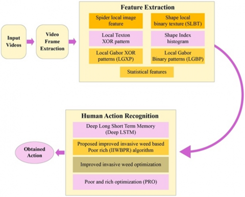
Aim is to provide a model for human action recognition with optimized Deep LSTM. The objective relies in devising an optimization driven technique for determining the actions of human considering a set of videos. At first, videos are collected, and subjected to video frame mining in which frames are mined using inputted video. Thereafter, the feature mining is executed to extract significant features from input video. Feature extraction helps to reduce dimensionality. Here, the features, like SLIF, SLBT, local Texton XOR pattern, LGBP [21], Shape Index histogram, LGXP [21] are extracted. Finally, the human action recognition is done using Deep LSTM [22] and its training is done using IIWBPR algorithm. The IIWBPR algorithm is devised by combining improved IWO [23] and PRO algorithm [24]. The configuration of human action recognition model with IIWBPR-based Deep LSTM is exemplified in Figure 1.
Figure 1. Human action recognition model with IIWBPR-based Deep LSTM
3.1 Acquire the input images
The first step in recognizing the actions of human from the videos is determining the actions from each frame of video. The actions in the videos represents that the person in videos are performing some kind of activity. Assume a video database M that contains r videos wherein persons are doing various activities and it can be modelled as:
$M=\left\{ {{F}_{1}},\,{{F}_{2}},\ldots ,{{F}_{t}},\ldots ,{{F}_{r}} \right\}$ (1)
where, Ft is tih video, and r refers total video count.
3.2 Obtain the video frames
Video comprises several frames and hence it is crucial to mine frames considering the videos for enhanced processing. Frames are extracted as one can discover the activity that occurs in the video just by observing few frames. Inputted video Ft is fed to video frame mining for extracting frames and each frame is employed by C and can be expressed by:
$C=\left\{ {{C}_{1}},\,{{C}_{2}},....{{C}_{p}},...{{C}_{q}} \right\}\,;\,{{C}_{p}}\in {{F}_{t}}$ (2)
where, Cp is mined frame from video Ft and q express total video frames count such that p= {1, 2, ..., q}.
3.3 Acquire vital features
Vital features are obtained from the video frames C wherein the apt features, namely SLIF, SLBT, Local Texton XOR patterns, LGBP, shape index histogram, LGXP and statistical features are obtained, and each feature are briefly exemplified below.
(i) SLIF
SLIF [25] represents feature descriptor, which considers an elite depiction sampling template using spider's orb-web model. A group of vectors $D=\left\{D^1, D^2, \ldots, D^\lambda\right\}$ linked to a group of targeted points $\left\{E 1, E_2, . ., E_\lambda\right\}$ from image. Each point $E_f$ is modelled through feature scale $\alpha_f$ and coordinate point $\left(l_f, m_f\right)$. At first, the orientation $\phi_f$ is allocated to each point $E_f \in E$. Then, an orb web model $Q_f$ is described for each point $E_a$. Web weights $K_f^{n, o}$ considers all web nodes $(n, o) f$. SLIF feature $D$ is obtained by combining 8-bit binary string series linked to its key point $E_a$ and can be expressed as:
${{D}_{f}}=\left[ \begin{align} & G_{1,1}^{f},G_{2,1}^{f},...,G_{n,1}^{f},G_{1,2}^{f},G_{2,2}^{f}, \\ & ...,G_{n,2}^{f},G_{1,2}^{f},G_{1,2}^{f},...,G_{n,o}^{f} \\\end{align} \right]$ (3)
where, $G_{n, o}^f$ expresses 8-bit binary array. The SLIF feature is designated as Q1.
(ii) SLBT
SLBT features [26] unifies both texture and shape information. Assume I=[I1, I2, .., Iu] be set of image provided u indicating total sets of training, and R=[R1, R2, .., Ru] represents shape landmark points. Thus, landmark points are assigned and alterations of shape are acquired wherein the shape vector R in training set is modelled by:
$R\approx \bar{R}+{{S}_{x}}{{T}_{x}}$ (4)
${{T}_{x}}=S_{x}^{N}(R-\bar{R})$ (5)
where, $\bar{R}$ represents mean shape, $T_x$ symbolize shape or weight attributes, $x$ depicts shape in $T_x, S_x$ represents eigen vector of highest eigen values. In addition, SLBT adapts LBP to acquire illumination and noise characteristics. The mining of LBP is quicker and simpler compared to Gabor wavelet. By considering the center pixel by $\left(\ell_j, \varpi_j\right)$ and intensity by $L_j$, function $A(b)$ is expressed as:
$A(b)=\left\{ \begin{align} & 1,\,\,\,\,\,\,\,b>0 \\ & 0,\,\,\,\,\,\,b\le 0 \\\end{align} \right.$ (6)
In center pixel, LBP is acquired as:
$LBP({{\ell }_{j}},{{\varpi }_{j}})=\sum\limits_{x=0}^{7}{H({{\ell }_{x}}}-{{\ell }_{j}}{{)}^{{{2}^{\ell }}}}$ (7)
where, $\ell_x$ represents grey values of eight adjoining pixels having $\ell_x(x=0,1,2,3,4,5,6,7)$. Assume $B=\left[B_l, B_2, \ldots, B_u\right]$ is employed as LBP feature histogram, which is trained. Modeling of Texture hence provided as:
${{T}_{y}}=S_{y}^{N}(B-\bar{B})$ (8)
where, Ty represents texture model, y signifies texture in Ty, eigen vector express Sy, and $\bar{B}$ defines mean vector. In addition, the shape and texture are produced by employing Principal Component Analysis (PCA) on unified vector attribute, which is provided by:
${{T}_{xy}}=\left( \begin{align} & {{H}_{x}}{{T}_{x}} \\ & \,\,\,{{T}_{y}} \\\end{align} \right)$ (9)
$D=S_{xy}^{N}({{T}_{xy}}-{{\bar{T}}_{xy}})$ (10)
where, Hx refers diagonal matrix, D stands for shape texture attribute, Sxy describes eigen vectors, and $\bar{T}_{x y}$ elucidates mean vector. SLBT feature is expressed as Q2.
(iii) Local XOR Texton pattern
The aim of Local XOR Texton pattern [27] is to categorize image textures and it is feasible to apply on various areas, like image retrieval and so on. It relies on correlation amidst the corresponding pixel and intermediate pixel in an image. The Local XOR Texton pattern is manipulated as:
${{\ell }_{X,Z}}=\sum\limits_{x=1}^{X}{{{2}^{(x-1)}}\times {{k}_{3}}\left( T({{q}_{j}})\otimes T\left( {{q}_{l}} \right) \right)}$ (11)
${{k}_{3}}\left( \nu \otimes \varepsilon \right)=\left\{ \begin{align} & 1\,\,\,\nu \ne \varepsilon \\ & 0\,\,else \\\end{align} \right.$ (12)
where, T(qj) exemplifies Texton shape for a neighbouring pixel qj and T(ql) stands for Texton shape for a neighbouring pixel ql and $\otimes$ symbolizes XOR operation amidst variables. The Local XOR Texton pattern feature is designated as Q3.
(iv) LGBP
LGBP [21] is acquired through encoding values of magnitude in LBP operator. Consider value of center by $\hbar_c$ and adjoining pixel by $\hbar_d$, then LGBP evaluation is manifested by:
$\Im \left( {{\hbar }_{d}}-{{\hbar }_{c}} \right)=\left\{ \begin{matrix} \begin{matrix} 1, & {{\hbar }_{d}}\ge {{\hbar }_{c}} \\\end{matrix} \\ \begin{matrix} 0, & {{\hbar }_{d}}<{{\hbar }_{c}} \\\end{matrix} \\\end{matrix} \right.$ (13)
In addition, the pattern of LBP with value of pixel is evaluated by allocating binomial factor d of each $\Im\left(\hbar_d-\hbar_c\right)$, and provided by:
$LBP=\sum\limits_{d=0}^{7}{\Im \left( {{\hbar }_{d}}-{{\hbar }_{c}} \right)\,{{2}^{d}}}$ (14)
Expression (14) depicts spatial pattern of local image texture. In addition, LGBP feature is expressed by Q4.
v) Shape index histogram
It represents an image geometry that captured second-order phase in continues time and permits one to analyze the curvature histogram distribution. The shape index histogram [28] is produced by selecting the group of nb bin centers b1bn consistently dispersed along the shape index interval π/2π/2. Considering a bin B centered at b, one can compute its total contributions considering the weighted sum of both curvedness metric c and spatial donut weighting D and is provided as:
$B\left( \sigma ,x,\gamma ,r,b,\beta \right)=\frac{\sum\nolimits_{x}{Dc\exp \left( -\frac{{{(b,s)}^{2}}}{2{{\beta }^{2}}} \right)}}{\sum\nolimits_{x}{D}}$ (15)
where, β symbolizes tonal scale parameter that helps to adjust smoothing, σ stands for scale, $s$ represents shape, and x,r,γ exemplifies spatial pooling. The shape index histogram feature is designated as Q5.
(vi) LGXP
LGXP [29] stages are firstly quantized to huge variety and then LXP operator is used for quantizing stages of innermost pixel and each of its neighbours. At last, the result binary labels are combined equally and local structures of central pixel. In addition, the patterns of LGXP in decimal and binary structure are expressed as:
$\begin{align} & {{\varepsilon }_{2}}={{\tau }_{\upsilon ,\kappa }}\left( {{\aleph }_{\nu }} \right) \\ & ={{\left[ \tau _{\upsilon ,\kappa }^{\beta },\tau _{\upsilon ,\kappa }^{\beta -1},...,\tau _{\upsilon ,\kappa }^{1} \right]}_{\eta }}={{\left[ \sum\limits_{\alpha =1}^{\beta }{{{2}^{\alpha -1}}}.\tau _{\upsilon ,\kappa }^{\alpha } \right]}_{\mu }} \\\end{align}$ (16)
where, $\eta$ expresses binary and $\mu$ is decimal, innermost pixel location in Gabor stage map with scale $v$ and orientation $\kappa$ is expressed by $\aleph_v$ while dimension of neighbourhood is expressed by $\beta$ and $\tau_{v, \kappa}^\alpha(\alpha=1,2, \ldots, \beta)$ indicates a structure evaluated amidst $\aleph_v$ and neighbour $\aleph_\alpha$, and represented as:
$\tau _{\upsilon ,\kappa }^{\alpha }=\vartheta \left( {{\theta }_{\upsilon ,\kappa }}\left( {{\aleph }_{\nu }} \right) \right)\otimes \vartheta \left( {{\theta }_{\upsilon ,\kappa }}\left( {{\aleph }_{\alpha }} \right) \right),\,\alpha =1,2,...,\beta $ (17)
where, θυ,κ(•) expresses phase, LXP operator is denoted as ⊗which is devised using XOR operator. ϑ(•) refers quantization operator which computes quantized code, which is modelled by:
$\nu \otimes \gamma =\left\{ \begin{align} & 0,\,\,\,\,\,\,\,if\,\nu =\gamma \\ & 1,\,\,\,\,\,\,\,\,\,\,else \\\end{align} \right.$ (18)
$\begin{align} & \vartheta \left( {{\theta }_{\upsilon ,\kappa }}\left( \bullet \right) \right)=\alpha ;\, \\ & \,if\,\frac{360*\alpha }{\partial }\le {{\theta }_{\upsilon ,\kappa }}\left( \bullet \right)<\frac{360*\left( \alpha +1 \right)}{\partial },\,\,\,\,\,\, \\ & \alpha =0,1,....,\partial -1 \\\end{align}$ (19)
where, $\partial$ represents number of phase ranges. The LGXP feature is designated as Q6.
(vii) Statistical features
Some of the statistical features adapted as imperative feature are listed:
(i) Mean
It exemplifies the complete values of images with respect to complete number of pixel values and it articulated as:
${{Q}_{7}}=\frac{1}{o}\sum\limits_{\psi =1}^{o}{{{\rho }_{\psi }}}$ (20)
where, o exposes total images count and number of pixel values is obtained as ρψ.
(ii) Variance
It indicates squared standard deviations wherein values of inputted image depicts variance and uttered as:
${{Q}_{8}}=ƛ_\chi^2=\frac{1}{o}\sum\limits_{\psi =1}^{o}{\left( {{\rho }_{\psi }}-{{Q}_{7}} \right)}$ (21)
where, Q7 specifies mean.
(iii) Standard deviation
It demonstrates variance square root, that can be modelled as:
${{Q}_{9}}=\sqrt{\frac{1}{o}\sum\limits_{\psi =1}^{o}{\left( {{\rho }_{\psi }}-{{Q}_{7}} \right)}}$ (22)
where, standard deviation is denoted by Q9.
(iv) Kurtosis
Statistical evaluated utilized for defining experimented distribution of image through a mean is termed as kurtosis and represented as:
${{Q}_{10}}=\frac{\sum{{{\left( {{Q}_{7}}-\overline{{{Q}_{7}}} \right)}^{4}}}}{o{{Q}_{9}}}$ (23)
where, Q7 is mean and Q9 expresses standard deviation.
(v) Skewness
It describes the quantification of distorted images from definite images and is modelled as:
${{Q}_{11}}=\frac{\sum\nolimits_{\psi }^{o}{\,\left( {{\xi }_{o}}-\overline{{{Q}_{7}}} \right)}}{\left( o-1 \right)*{{Q}_{10}}}$ (24)
where, o defines number of images, ξo reveals arbitrarily selected image. Hence, the obtained feature vector is manipulated as:
$Q=\{{{Q}_{1}},{{Q}_{2}},\ldots ,{{Q}_{11}}\}$ (25)
3.4 Recognition of human activity using IIWBPR-based Deep LSTM
The human activity is recognized considering the IIWBPR-Deep LSTM which is trained with IIWBPR with feature vector Q. The deep LSTM has the capability for learning the features automatically from the raw sensor data. Here, the IIWBPR is obtained by unifying the merits of both IWO and PRO algorithm. Deep LSTM and IIWBPR steps are defined herewith.
a) Deep LSTM structure
Deep LSTM [30] is employed for managing diminution and assortment of data by utilizing using feature vector Q and input parameter set U. The inputted node Ve adapts input U using deep input and through hidden states ae-1. Thus, the data forecast becomes non-linear, and hence technique employed to evaluate output is termed to be non-linear, that offers output with highest accuracy. The outcome of cluster-assisted topology routing U and ae-1 is fed to tanh function is represented as:
${{V}_{e}}=\tanh \left( \delta .{{g}_{V\delta }}+{{O}_{e-1}}{{g}_{V\delta }}+{{P}_{sa}} \right)$ (26)
where, gVδ depicts weight matrix, Oe-1 displays input of hidden state, and Psa signifies bias to inputted node.
Input gate process is represented as:
$\mathrm{T}_e=\lambda\left(\delta \cdot g_{V \delta}+a_{e-1} g_{V a}+P_s\right)$ (27)
where, Te refers inputted gate at instance e, λ signifies sigmoidal activation function, and Ps denotes bias to inputted gate and is provided by:
$\mathrm{T}_e=\lambda\left(\delta \cdot g_{V \delta}+a_{e-1} g_{V a}+P_s\right)$ (28)
where, Ve is interior state at instance e, and ke-1 is internal state at instance e-1. The forget gate W is utilized to reinitiate memory cell internal state, and definedby:
${{W}_{e}}=\lambda \left( \delta .{{g}_{W\delta }}+{{a}_{e-1}}{{g}_{Ws}}+{{P}_{f}} \right)$ (29)
where, W refers forget state at instance $e$, Θ signifies linear operator, gWδ stands for weight among forget and input layer, gWs symbolizes weight among forget and hidden state, and Pf depicts forget gate bias.
Output gate Oe is presented by:
${{O}_{e}}=\lambda \left( e.{{g}_{a\delta }}+{{a}_{e-1}}{{g}_{Oa}}+{{P}_{o}} \right)$ (30)
where, gaδ exemplifies weight among output and input layers, gOa denotes weight amidst output and hidden states, and Po denotes output gate bias.
Furthermore, the finalized output obtained through memory cell is manifested by:
${{a}_{e}}=\tanh \left( {{k}_{e}} \right)\Theta {{O}_{e}}$ (31)
b) Training with IIWBPR
Deep LSTM training is implemented with IIWBPR wherein is generated by combining IWO and PRO. IWO [23] represents population-assisted evolutionary technique motivated from weed colony features. It relies on chaos theory, which aids to attain a quick rate of convergence and elevated accuracy. It maximizes population diversity and is utilized to update location to weed. It uses sigma that helps to create quick variations over the iterations. On the other hand, the PRO [24] is obtained by two sets of poor and rich that tries to attain wealth and enhance its economic conditions. It had effective performance in solving the real-time problems and finds best parameter values. It discovers optimum parameters by controlling the conditions of each problem. Hence, the incorporation of PRO in IWO is done to improve whole performance. Hence, developed IIWBPR steps are described herewith.
Step 1: Initialization
Fundamental step includes initialization of solution and expressed as Y with total Ψ solution such that 1≤Φ≤Ψ.
$Y=\{{{Y}_{1}},{{Y}_{2}},\ldots ,{{Y}_{\Phi }},\ldots ,{{Y}_{\Psi }}\}$ (32)
where, Ψ depicts total solution, and YΦ referred Φth solution.
Step 2: Locate error
The error is generated based on mean square error and the optimal results are obatined based on the minimum error value.
$E r r=\frac{1}{\mathrm{E}} \sum_{o=1}^{\mathrm{E}}\left[\varpi_o-O\right]^2$ (33)
where, Err is error function, E expresses total instances, ϖο defines predicted output, and O is Deep LSTM output.
Step 3: Specify logistic chaotic map
According to IWO [23], the admired chaotic maps indicates logistic chaotic map and is employed as a second order polynomial and this logistic chaotic map is represented by:
${{Y}_{h+1}}=v{{Y}_{h}}(1-{{Y}_{h}})$ (34)
where, v is capricious number and Yh is arbitrary number amidst [0, 1]. Hence 0<v≤4, and h=0, 1, 2, … and Yh∈[0,1].
According to IWO, the optimum weed is utilized to finest solution and is represented by:
$Y_{w}^{z+1}=\chi (z)\times Y_{w}^{z}+({{Y}_{best}}-Y_{w}^{z})$ (35)
where, $Y_w^{z+1}$ depicts new weed location, $Y_w^z$ reveals current weed location, Ybest denotes best weed discovered, and χ(z) expose presents standard deviation.
The standard deviation is provided by:
$\begin{align} & \chi (z)={{\left( \frac{Z-z}{Z} \right)}^{v}}\left( {{\chi }_{initial}}-{{\chi }_{final}} \right) \\ & +{{\chi }_{final}}\times \gamma (z) \\\end{align}$ (36)
where, γ(z) refers chaotic mapping in zth iteration, Z indicates highest iteration.
$Y_{w}^{z+1}=Y_{w}^{z}(\chi (z)-1)+{{Y}_{best}}$ (37)
For obtaining better efficiency, PRO is used. According to PRO [24], the update expression is manifested by:
$\vec{Y}_{rich,z}^{new}=\vec{Y}_{rich,z}^{old}+i\left( \vec{Y}_{rich,z}^{old}-\vec{Y}_{poor,best}^{old} \right)$ (38)
where, $i$ stands for class gap parameter, $\vec{Y}_{\text {poor,best }}^{\text {old }}$ is present position of best member of the poor population, $\vec{Y}_{\text {rich }, z}^{o l d}$ stands for present position of rich member and $\vec{Y}_{r i c h, z}^{n e w}$ is new position of rich member.
Assume $\vec{Y}_{\text {rich }, z}^{\text {new }}=Y_z^{w+1}$ and $\vec{Y}_{\text {rich }, z}^{\text {old }}=Y_z^w$ and $\vec{Y}_{\text {poor }, \text { best }}^{\text {old }}=$ $Y_{\text {pbest }}^w$
Now equation becomes:
$Y_{z}^{w+1}=Y_{z}^{w}+i\left( Y_{z}^{w}-Y_{pbest}^{w} \right)$ (39)
$Y_{z}^{w+1}=Y_{z}^{w}+iY_{z}^{w}-iY_{pbest}^{w}$ (40)
$Y_{z}^{w+1}=Y_{z}^{w}\left( 1+i \right)-iY_{pbest}^{w}$ (41)
$Y_{z}^{w}=\frac{Y_{z}^{w+1}+iY_{pbest}^{w}}{1+i}$ (42)
Substitute expression (42) in expression (37):
$Y_{w}^{z+1}=\left[ \frac{Y_{z}^{w+1}+iY_{pbest}^{w}}{1+i} \right](\chi (z)-1)+{{Y}_{best}}$ (43)
$\begin{align} & Y_{w}^{z+1}=\frac{Y_{z}^{w+1}}{1+i}(\chi (z)-1) \\ & +\left[ \frac{iY_{pbest}^{w}}{1+i} \right](\chi (z)-1)+{{Y}_{best}} \\\end{align}$ (44)
$\begin{align} & Y_{w}^{z+1}-\frac{Y_{z}^{w+1}}{1+i}(\chi (z)-1) \\ & =\left[ \frac{iY_{pbest}^{w}}{1+i} \right](\chi (z)-1)+{{Y}_{best}} \\\end{align}$ (45)
$\begin{align} & Y_{w}^{z+1}\left[ 1-\frac{(\chi (z)-1)}{1+i} \right] \\ & =\left[ \frac{iY_{pbest}^{w}}{1+i} \right](\chi (z)-1)+{{Y}_{best}} \\\end{align}$ (46)
$\begin{align} & Y_{w}^{z+1}\left[ \frac{1+i-\chi (z)+1}{1+i} \right] \\ & =\left[ \frac{iY_{pbest}^{w}}{1+i} \right](\chi (z)-1)+{{Y}_{best}} \\\end{align}$ (47)
$\begin{align} & Y_{w}^{z+1}\left[ \frac{2+i-\chi (z)}{1+i} \right] \\ & =\left[ \frac{iY_{pbest}^{w}}{1+i} \right](\chi (z)-1)+{{Y}_{best}} \\\end{align}$ (48)
$\begin{align} & Y_{w}^{z+1}\left[ 2+i-\chi (z) \right] \\ & =\left[ iY_{pbest}^{w} \right](\chi (z)-1)+(1+i){{Y}_{best}} \\\end{align}$ (49)
Thus, the update expression of IIWBPR is given as:
$Y_{w}^{z+1}=\frac{iY_{pbest}^{w}(\chi (z)-1)+{{Y}_{best}}(1+i)}{2+i-\chi (z)}$ (50)
Step 4: Re-estimate error to generate optimum solution
The most favourable solution is enumerated with error, and solution having least error is known as finest solution.
Step 5: Termination
Aforesaid steps are repeated until highest iteration is attained to expose finest solution. The pseudo-code of IIWBPR is elucidated in Table 1.
Table 1. Pseudo code of IIWBPR
|
Input: $Y$: Solution group, $z$: prior iteration, $Z$: elevated iteration |
|
Output: Finest solution ${{Y}_{best}}$ |
|
Begin |
|
Construct arbitrary population $Y$. |
|
Initiate other attributes, such $\chi (z)$ |
|
Find error with expression (33) |
|
For $z=1\,to\,Z$ |
|
For each individual $w\in \varpi $ |
|
Specify seed count for $w$ with error |
|
Capriciously hand out seeds on search space |
|
Adjoin generated seeds to solution set $w$ |
|
If $(|w|=\omega )>{{\varpi }_{\max }}$ |
|
Sort using expression (50) |
|
Trim population having less fitness value till $\omega =Z$ |
|
End if |
|
End for |
|
End for |
|
Return ${{Y}_{best}}$ |
|
$z=z+1$ |
|
End |
Propensity of IIWBPR-Deep LSTM is examined by checking the quality of each method with certain metrics by altering K-set and training data.
4.1. Setup of experiments
Functioning of IIWBPR-Deep LSTM is implemented in PYTHON.
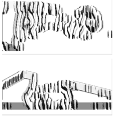
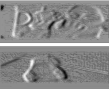
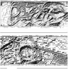
a) Input images
b) LGBP images
c) LGXP images
d) LTXORPs images
e) SLBT images
Figure 2. Experimental outcomes of proposed IIWBPR+Deep LSTM
4.2 Dataset description
The dataset considered for analysis is UCF101 videos dataset [31]. This dataset contains original UCF101 videos. It is offered by Center for Research in Computer Vision. It represents an action recognition database that poses real action videos and has 101 action categories. It contains 13320 video clips and are splitted into 101 classes.
4.3 Experimental outcomes
Figure 2 exemplifies the experimental upshots of IIWBPR+Deep LSTM using set of images.
4.4 Performance metrics
Qualities of each approach are calculated with specific measures and are elucidated below.
4.4.1 Accuracy
It defined the degree of computed value to its real value in recognizing the human action and is manipulated as:
$A^{c y}=\frac{\partial^p+\lambda^n}{\partial^p+\partial^n+\lambda^p+\lambda^n}$ (51)
where, ∂p stands for true positive, ∂n portray true negative, λp be false positive, and λn symbolize false negative.
4.4.2 Sensitivity
It depicts fraction of positives which is identified by action recognition model accurately, and can be manifested as:
$S^{t y}=\frac{\partial^p}{\partial^p+\lambda^n}$ (52)
4.4.3 Specificity
It depicts fraction of negatives determined with designed model accurately, and can be manifested as:
$S^{p y}=\frac{\partial^n}{\partial^n+\lambda^p}$ (53)
4.4.4 F1-Score
The harmonic mean of recall and precision is the F1 score. It is a statistical metric used to evaluate performance.
4.5 Performance assessment
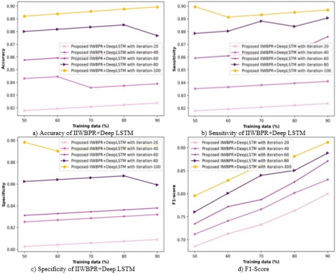
Figure 3 portrays the analysis of IIWBPR+Deep LSTM performance using distinct measures. The accuracy related study is exhibited in figure 3a). For 50% training data, the accuracy observed by IIWBPR+Deep LSTM using iteration 20 to 100 are 0.818, 0.843, 0.858, 0.880, and 0.892. Moreover for 90% training data, the accuracy observed by proposed IIWBPR+Deep LSTM using iteration 20 to 100 are 0.824, 0.839, 0.864, 0.877, and 0.899. The sensitivity related analysis is exhibited in figure 3b). For 50% training data, the sensitivity observed by IIWBPR+Deep LSTM using iteration 20 to 100 are 0.818, 0.835, 0.859, 0.879, and 0.899. Moreover for 90% training data, the sensitivity observed by IIWBPR+Deep LSTM using iteration 20 to 100 are 0.824, 0.841, 0.876, 0.891, and 0.897. The specificity related analysis is exhibited in figure 3c). For 50% training data, the specificity observed by proposed IIWBPR+Deep LSTM using iteration 20 to 100 are 0.803, 0.825, 0.831, 0.862, and 0.898. Moreover for 90% training data, the specificity observed by IIWBPR+Deep LSTM using iteration 20 to 100 are 0.809, 0.832, 0.838, 0.859, and 0.896. The F1-score related analysis is exhibited in figure 3d). For 50% training data, the F1-score observed by proposed IIWBPR+Deep LSTM using iteration 20 to 100 are 0.685, 0.712, 0.734, 0.760, and 0.795. Moreover for 90% training data, the F1-score observed by IIWBPR+Deep LSTM using iteration 20 to 100 are 0.799, 0.830, 0.870, 0.888, and 0.911.
Figure 3. Analysis of performance assessment
4.6 Algorithm techniques
Algorithms engaged for analysis includes WOA+Deep LSTM [32], NBO+Deep LSTM [33], IIWA+Deep LSTM [22, 23], PRO+Deep LSTM [22, 24], and IIWBPR+Deep LSTM.
4.7 Algorithm analysis
Algorithmic analysis is executed by adapting distinct measures and by changing iterations.
Figure 4. Various algorithms of analysis
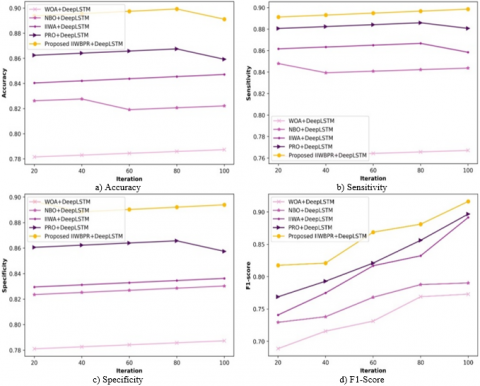
The illustration regarding the algorithmic analysis considering distinct metrics is explained in figure 4. The accuracy analysis is exemplified in figure 4a). Allowing 20 iterations, the accuracy observed by WOA+Deep LSTM, NBO+Deep LSTM, IIWA+Deep LSTM, PRO+Deep LSTM are 0.782, 0.826, 0.840, 0.862, whereas accuracy of IIWBPR+Deep LSTM is 0.894. Also considering 100 iterations, the accuracy observed by WOA+Deep LSTM, NBO+Deep LSTM, IIWA+Deep LSTM, PRO+Deep LSTM are 0.787, 0.822, 0.847, 0.859, whereas accuracy of IIWBPR+Deep LSTM is 0.891. The enhancement in performance in view of existing with proposed using accuracy is 11.672%, 7.744%, 4.938%, 3.591%. The sensitivity analysis is exhibited in figure 4b). Allowing 20 iterations, the sensitivity observed by WOA+Deep LSTM, NBO+Deep LSTM, IIWA+Deep LSTM, PRO+Deep LSTM are 0.761, 0.848, 0.862, 0.881, whereas sensitivity of IIWBPR+Deep LSTM is 0.891. The specificity related analysis is exhibited in figure 4c). Allowing 20 iterations, the specificity observed by WOA+Deep LSTM, NBO+Deep LSTM, IIWA+Deep LSTM, PRO+Deep LSTM are 0.781, 0.824, 0.830, 0.861, whereas specificity of IIWBPR+Deep LSTM is 0.897. Also considering 100 iterations, the specificity observed by WOA+Deep LSTM, NBO+Deep LSTM, IIWA+Deep LSTM, PRO+Deep LSTM are 0.787, 0.830, 0.836, 0.857, whereas specificity of IIWBPR+Deep LSTM is 0.894. The enhancement in performance in view of existing with proposed using specificity is 11.968%, 7.158%, 6.487%, 4.138%. The F1-score related analysis is exhibited in figure 5d). Allowing 20 iterations, the F1-score observed by WOA+Deep LSTM, NBO+Deep LSTM, IIWA+Deep LSTM, PRO+Deep LSTM are 0.688, 0.729, 0.740, 0.768, whereas F1-score of IIWBPR+Deep LSTM is 0.817. Also considering 100 iterations, the F1-score observed by WOA+Deep LSTM, NBO+Deep LSTM, IIWA+Deep LSTM, PRO+Deep LSTM are 0.772, 0.790, 0.891, 0.896, whereas specificity of IIWBPR+Deep LSTM is 0.916. The enhancement in performance in view of existing with proposed using F1-score is 15.72%, 13.75%, 2.72%, 2.18%.
4.8 Comparative methods
Approaches employed for analysis involves M-SVM, DNN, LSTM, PCANET, Deep LSTM, and IIWBPR-Deep LSTM.
4.9 Comparative assessment
Approaches analysis is implemented by altering x-axis values with training data and K-set (Testing data).
(a) Training data evaluation
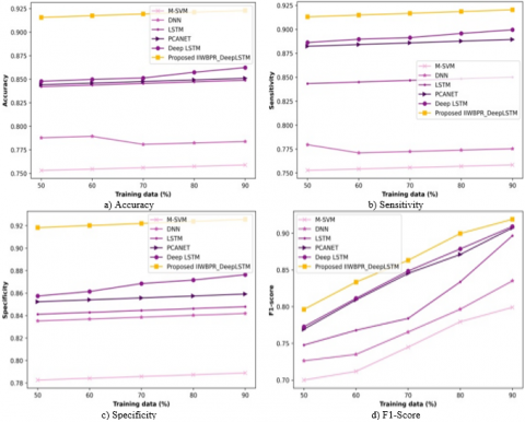
Figure 5 demonstrates approaches analysis by changing training data on x-axis. The accuracy-based study is demonstrated in Figure 5a). With 50% training data, the utmost accuracy of 0.916 is observed by IIWBPR-Deep LSTM while accuracy of M-SVM, DNN, LSTM, PCANET, and Deep LSTM are 0.753, 0.788, 0.842, 0.844, and 0.848. Besides with 90% training data, the utmost accuracy of 0.923 is observed by IIWBPR-Deep LSTM while accuracy of M-SVM, DNN, LSTM, PCANET, and Deep LSTM are 0.759, 0.784, 0.849, 0.851, and 0.862. The enhancement in performance considering existing with IIWBPR-Deep LSTM using accuracy is 17.768%, 15.059%, 8.017%, 7.800%, and 6.609%. The sensitivity analysis is demonstrated in Figure 5b). With 50% training data, the utmost sensitivity of 0.913 is observed by IIWBPR-Deep LSTM while sensitivity of M-SVM, DNN, LSTM, PCANET, and Deep LSTM are 0.753, 0.780, 0.843, 0.882, and 0.886. Besides with 90% training data, the utmost sensitivity of 0.920 is observed by IIWBPR-Deep LSTM while sensitivity of M-SVM, DNN, LSTM, PCANET, and Deep LSTM are 0.759, 0.775, 0.850, 0.889, and 0.900. The enhancement in performance considering existing with IIWBPR-Deep LSTM using sensitivity is 17.5%, 15.760%, 7.608%, 3.369%, and 2.174%. The specificity analysis is demonstrated in Figure 5c). With 50% training data, the utmost specificity of 0.918 is observed by IIWBPR-Deep LSTM while specificity of M-SVM, DNN, LSTM, PCANET, and Deep LSTM are 0.783, 0.835, 0.841, 0.852, and 0.857. Besides with 90% training data, the utmost specificity of 0.926 is observed by IIWBPR-Deep LSTM while specificity of M-SVM, DNN, LSTM, PCANET, and Deep LSTM are0.789, 0.842, 0.848, 0.859, and 0.876. The enhancement in performance considering existing with IIWBPR-Deep LSTM using specificity is14.794%, 9.071%, 8.423%, 7.235%, and 5.400%. The F1-score analysis is demonstrated in Figure 5d). With 50% training data, the utmost F1-score of 0.796 is observed by IIWBPR-Deep LSTM while F1-score of M-SVM, DNN, LSTM, PCANET, and Deep LSTM are 0.699, 0.726, 0.747, 0.769, and 0.773. Besides with 90% training data, the utmost F1-score of 0.919 is observed by IIWBPR-Deep LSTM while F1-score of M-SVM, DNN, LSTM, PCANET, and Deep LSTM are 0.799, 0.835, 0.896, 0.907, and 0.909. The enhancement in performance considering existing with IIWBPR-Deep LSTM using F1-score is 13.05%, 9.14%, 2.50%, 1.30%, and 1.088%.
Figure 5. Analysis of approaches with training data
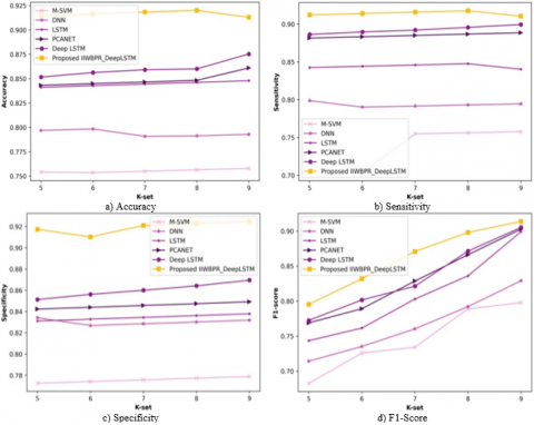
Figure 6. Analysis of approaches with K-set
(b) K-set evaluation
Figure 6 renders the analysis of approaches by changing K-set values on x-axis. The accuracy assessment graph is rendered in Figure 6a). Allowing K-set=5, the accuracy observed by M-SVM is 0.754, DNN is 0.797, LSTM is 0.841, PCANET is 0.843, Deep LSTM is 0.852, and IIWBPR-Deep LSTM is 0.915. Furthermore, allowing K-set=9, the accuracy noted by M-SVM is 0.758, DNN is 0.793, LSTM is 0.848, PCANET is 0.861, Deep LSTM is 0.875 and IIWBPR-Deep LSTM is 0.913. The enhancement in performance in view of existing with proposed using accuracy is 16.976%, 13.143%, 7.119%, 5.695%, and 4.162%. The sensitivity related analysis is exhibited in Figure 6b). Allowing K-set=5, the sensitivity observed by M-SVM is 0.752, DNN is 0.799, LSTM is 0.843, PCANET is 0.882, Deep LSTM is 0.886, and IIWBPR-Deep LSTM is 0.912. Furthermore, considering K-set=9, the sensitivity observed by M-SVM is 0.758, DNN is 0.795, LSTM is 0.840, PCANET is 0.889, Deep LSTM is 0.900, and IIWBPR-Deep LSTM is 0.911. The enhancement in performance in view of existing with proposed using sensitivity is 16.794%, 12.733%, 7.793%, 2.414%, and 1.207%. The specificity related analysis is exhibited in Figure 6c). Allowing K-set=5, the specificity observed by M-SVM is0.773, DNN is 0.834, LSTM is 0.831, PCANET is 0.842, Deep LSTM is 0.851 and proposed IIWBPR-Deep LSTM is 0.917. Furthermore, considering K-set=9, the specificity observed by M-SVM is 0.779, DNN is 0.832, LSTM is 0.838, PCANET is 0.849, Deep LSTM is 0.870 and IIWBPR-Deep LSTM is 0.925. The enhancement in performance in view of existing with proposed using specificity is 15.783%, 10.054%, 9.405%, 8.216%, and 5.946%. The F1-Score related analysis is exhibited in Figure 6d). Allowing K-set=5, the F1-Score observed by M-SVM is0.682, DNN is 0.714, LSTM is 0.743, PCANET is 0.768, Deep LSTM is 0.772, and proposed IIWBPR-Deep LSTM is 0.795. Furthermore, considering K-set=9, the F1-Score observed by M-SVM is 0.797, DNN is 0.829, LSTM is 0.899, PCANET is 0.902, Deep LSTM is 0.905, and IIWBPR-Deep LSTM is 0.913. The enhancement in performance in view of existing with proposed using F1-Score is 12.70%, 9.20%, 1.53%, 1.20%, and 0.985%.
4.10 Comparative discussion
The assessment is executed with algorithms and techniques using distinct metrics.
a) Algorithm analysis
Table 2 represents algorithmic analysis considering several algorithms with Deep KSTM. Supreme accuracy of 89.1% is produced by IIWBPR+ Deep LSTM whereas accuracy of existing is 78.7%, 82.2%, 84.7% and 85.9%. The highest sensitivity of 89.9% is noted by IIWBPR+ Deep LSTM whereas accuracy of existing is 76.7%, 84.4%, 85.8% and 88.1%. The highest specificity of 89.4% is obtained by IIWBPR+ Deep LSTM whereas accuracy of existing is 78.7%, 83%, 83.6% and 85.7%.
b) Approach analysis
Table 3 demonstrates approach analysis by changing training data and K-set in x-axis. With training data, the supreme accuracy of 92.3%, sensitivity of 92% and specificity of 92.6% is noted by IIWBPR+ Deep LSTM. With K-set, the supreme accuracy of 91.3%, sensitivity of 91.1% and specificity of 92.5% is noted by IIWBPR+ Deep LSTM.
Table 2. Comparing with Various approaches of Algorithms analysis with our proposed IIWBPR+Deep LSTM
|
Metrics |
WOA+ Deep LSTM |
NBO+ Deep LSTM |
IIWA+ Deep LSTM |
PRO+ Deep LSTM |
Proposed IIWBPR+Deep LSTM |
|
Accuracy (%) |
78.7 |
82.2 |
84.7 |
85.9 |
89.1 |
|
Sensitivity (%) |
76.7 |
84.4 |
85.8 |
88.1 |
89.9 |
|
Specificity (%) |
78.7 |
83 |
83.6 |
85.7 |
89.4 |
|
F1-Score |
77.2 |
79 |
89.1 |
89.6 |
91.6 |
Table 3. Approach analysis
|
Metrics |
M-SVM |
DNN |
LSTM |
PCA NET |
Deep LSTM |
Proposed IIWBPR-Deep LSTM |
|
Training data (%) |
||||||
|
Accuracy (%) |
75.9 |
78.4 |
84.9 |
85.1 |
86.2 |
92.3 |
|
Sensitivity (%) |
75.9 |
77.5 |
85 |
88.9 |
90.0 |
92 |
|
Specificity (%) |
78.9 |
84.2 |
84.8 |
85.9 |
87.6 |
92.6 |
|
F1-Score |
79.9 |
83.5 |
89.6 |
90.7 |
90.9 |
91.9 |
|
K-set |
||||||
|
Accuracy (%) |
75.8 |
79.3 |
84.8 |
86.1 |
87.5 |
91.3 |
|
Sensitivity (%) |
75.8 |
79.5 |
84 |
88.9 |
90.0 |
91.1 |
|
Specificity (%) |
77.9 |
83.2 |
83.8 |
84.9 |
87.0 |
92.5 |
|
F1-Score |
79.7 |
82.9 |
89.9 |
90.2 |
90.5 |
91.3 |
The detection of actions amidst the set of humans is essential and tends to be a necessary domain in the vicinity of artificial intelligence. An optimized deep model is presented for HAR. The main contribution is to provide optimization assisted model for determining actions of human considering a set of videos. Input video are accumulated, and it undergoes video frame extraction wherein frames are obtained through inputted video. Thereafter, the feature mining is done to attain significant features using inputted video. Here, the features, like SLBT, local Texton XOR pattern, LGBP, Shape Index histogram, LGXP and statistical features are produced. The learned features are further used to train Deep LSTM classifier for recognizing the actions. HAR is implemented with Deep LSTM, which is further trained with IIWBPR algorithm. The IIWBPR algorithm is produced by blending IIWO and PRO. The IIWBPR-assisted Deep LSTM outperformed with supreme accuracy of 92.3%, sensitivity of 92%, specificity of 92.6% and F1 Score of 91.9%. Thus, the proposed IIWBPR- Deep LSTM offered superior efficiency in detecting the human actions. The devised IIWBPR+Deep LSTM is used in various sectors, like sports performance analysis, healthcare, intelligent monitoring, gaming, etc. However, large dataset is not considered for validating the performance of the proposed model. Future works covers implementation with other datasets to validate feasibility of designed model.
[1] Baccouche, M., Mamalet, F., Wolf, C., Garcia, C., Baskurt, A. (2011). Sequential deep learning for human action recognition. In Proceedings of International Workshop on Human Behavior Understanding, pp. 29-39. https://doi.org/10.1007/978-3-642-25446-8_4
[2] Yeffet, L., Wolf, L. (2003). Local trinary patterns for human action recognition. In Proceedings of IEEE 12th International Conference on Computer Vision, pp. 492-497. https://doi.org/10.1109/ICCV.2009.5459201
[3] Kong, Y., Fu, Y. (2022). Human action recognition and prediction: A survey. International Journal of Computer Vision, 130(5): 1366-1401. 10.1007/s11263-022-01594-9
[4] Zhang, H.B., Zhang, Y.X., Zhong, B., Lei, Q., Yang, L., Du, J.X., Chen, D.S. (2019). A comprehensive survey of vision-based human action recognition methods. Sensors, 19(5): 1005. https://doi.org/10.3390/s19051005
[5] Masoud, O., Papanikolopoulos, N. (2003). A method for human action recognition. Image and Vision Computing, 21(8):729-743. https://doi.org/10.1016/S0262-8856(03)00068-4
[6] Vemulapalli, R., Arrate, F., Chellappa, R. (2014). Human action recognition by representing 3d skeletons as points in a lie group. In Proceedings of the IEEE Conference on Computer Vision and Pattern Recognition, Columbus, OH, USA, pp. 588-595. https://doi.org/10.1109/CVPR.2014.82
[7] Shao, L., Zhen, X.T., Tao, D.C., Li, X.L. (2014). Spatiotemporal Laplacian pyramid coding for action recognition. IEEE Transactions on Cybernetics, 44(6): 817-827. https://doi.org/10.1109/TCYB.2013.2273174
[8] Burghouts, G. J., Schutte, K., ten Hove, R. J. M., van den Broek, S. P., Baan, J., Rajadell, O., Ferryman, J. (2014). Instantaneous threat detection based on a semantic representation of activities, zones and trajectories. Signal, Image and Video Processing, 8: 191-200. https://doi.org/10.1007/s11760-014-0672-1
[9] Yang, X., Tian, Y.L. (2014). Super normal vector for activity recognition using depth sequences. In Proceedings of IEEE Conference on Computer Vision and Pattern Recognition, pp. 804-811.
[10] Li, M., Leung, H., Shum, H.P.H. (2016). Human action recognition via skeletal and depth based feature fusion. In Proceedings of the Motion in Games, pp. 123-132. https://doi.org/10.1145/2994258.2994268
[11] Wang, J., Liu, Z., Wu, Y., Yuan, J. (2013). Learning actionlet ensemble for 3D human action recognition. IEEE Transactions on Pattern Analysis and Machine Intelligence, 36(5): 914-927. https://doi.org/10.1109/TPAMI.2013.198
[12] Simonyan, K., Zisserman, A. (2014). Two-stream convolutional networks for action recognition in videos. In Proceedings of the NIPS Neural Information Processing Systems Conference, pp. 568-576.
[13] Khan, M.A., Sharif, M., Akram, T., Raza, M., Saba, T., Rehman, A. (2022). Hand-crafted and deep convolutional neural network features fusion and selection strategy: An application to intelligent human action recognition. Applied Soft Computing, 87: 105986. https://doi.org/10.1016/j.asoc.2019.105986
[14] Khan, M.A., Javed, K., Khan, S.A., Saba, T., Habib, U., Khan, J.A., Abbasi, A.A. (2020). Human action recognition using fusion of multiview and deep features: An application to video surveillance. Multimedia Tools and Applications, 1-27. https://doi.org/10.1007/s11042-020-08806-9
[15] Dai, C., Liu, X., Lai, J. (2020). Human action recognition using two-stream attention based LSTM networks. Applied soft computing, 86: 105820. https://doi.org/10.1016/j.asoc.2019.105820
[16] Jaouedi, N., Boujnah, N., Bouhlel, M.S. (2020). A new hybrid deep learning model for human action recognition. Journal of King Saud University-Computer and Information Sciences, 32(4): 447-453. https://doi.org/10.1016/j.jksuci.2019.09.004
[17] Abdelbaky, A., Aly, S. (2020). Human action recognition using short-time motion energy template images and PCANet features. Neural Computing and Applications, 1-14. https://doi.org/10.1007/s00521-020-04712-1
[18] Ozcan, T., Basturk, A. (2020). Human action recognition with deep learning and structural optimization using a hybrid heuristic algorithm. Cluster Computing, 1-14. https://doi.org/10.1007/s10586-020-03050-0
[19] Majd, M., Safabakhsh, R. (2020). Correlational convolutional LSTM for human action recognition. Neurocomputing, 396: 224-229. https://doi.org/10.1016/j.neucom.2018.10.095
[20] He, J.Y., Wu, X., Cheng, Z.Q., Yuan, Z., Jiang, Y.G. (2021). DB-LSTM: Densely-connected Bi-directional LSTM for human action recognition. Neurocomputing, 444: 319-331. https://doi.org/10.1016/j.neucom.2020.05.118
[21] Zhang, W., Shan, S., Gao, W., Chen, X., Zhang, H. (2005). Local gabor binary pattern histogram sequence (lgbphs): A novel non-statistical model for face representation and recognition. In Tenth IEEE International Conference on Computer Vision (ICCV'05), pp.786-791. https://doi.org/10.1109/ICCV.2005.147
[22] JeyanthiSuresh, A., Visumathi, J. (2020). Inception ResNet deep transfer learning model for human actionrecognition using LSTM, Materialstoday Proceedings.
[23] Zheng, Z.X., Li, J.Q. (2018). Optimal chiller loading by improved invasive weed optimization algorithm for reducing energy consumption. Energy and Buildings, 161: 80-88. https://doi.org/10.1016/j.enbuild.2017.12.020
[24] Moosavi, S.H.S., Bardsiri, V.K. (2019). Poor and rich optimization algorithm: A new human-based and multi populations algorithm. Engineering Applications of Artificial Intelligence, 86: 165-181. https://doi.org/10.1016/j.engappai.2019.08.025
[25] Fausto, F., Cuevas, E., Gonzales, A. (2017). A new descriptor for image matching based on bionic principles. Pattern Analysis and Applications, 20: 1245-1259. https://doi.org/10.1007/s10044-017-0605-z
[26] Lakshmiprabha, N.S., Majumder, S. (2012). Face recognition system invariant to plastic surgery. In 2012 12th International Conference on Intelligent Systems Design and Applications (ISDA), pp. 258-263. https://doi.org/10.1109/ISDA.2012.6416547
[27] Anandababu, P., Kamarasan, M. (2020). Quadhistogram with local texton xor patterns based feature extraction for content based image retreival system. The International Journal of Analytical and Experimental Modal Analysis, 12(2).
[28] Larsen, A.B.L., Vestergaard, J.S., Larsen, R. (2014). HEp-2 cell classification using shape index histograms with donut-shaped spatial pooling. IEEE Transactions on Medical Imaging, 33(7): 1573-1580. https://doi.org/10.1109/TMI.2014.2318434
[29] Xie, S., Shan, S., Chen, X., Chen, J. (2010). Fusing local patterns of gabor magnitude and phase for face recognition. IEEE Transactions on Image Processing, 19(5): 1349-1361. https://doi.org/10.1109/TIP.2010.2041397
[30] Majhi, B., Naidu, D., Mishra, A.P., Satapathy, S.C. (2020). Improved prediction of daily pan evaporation using Deep-LSTM model. Neural Computing and Applications, 32: 7823-7838. https://doi.org/10.1007/s00521-019-04127-7
[31] UCF101dataset. https://www.kaggle.com/datasets/pevogam/ucf101, Accessed on July 2022.
[32] Mirjalili, S., Lewis, A. (2016). The whale optimization algorithm. Advances in Engineering Software, 95: 51-67. https://doi.org/10.1016/j.advengsoft.2016.01.008
[33] Chahardoli, M., Eraghi, N.O., Nazari, S. (2022). Namib beetle optimization algorithm: A new meta‐heuristic method for feature selection and dimension reduction. Concurrency and Computation: Practice and Experience, 34(1): 6524. https://doi.org/10.1002/cpe.6524