Nataliya Boyko![]()
© 2023 IIETA. This article is published by IIETA and is licensed under the CC BY 4.0 license (http://creativecommons.org/licenses/by/4.0/).
OPEN ACCESS
The objective of this study was to conduct a comprehensive evaluation of binary classification algorithms within data lakes, employing a diverse array of metrics. Binary classification algorithms, which categorize inputs into one of two distinct classes, were scrutinized to determine their efficacy. The research focused on the evaluation techniques applicable to these algorithms. Methods for assessing algorithmic efficiency were investigated, including logistic regression, error function, regularization, and ancillary training tools within the dataset. A detailed analysis of the parameters pertinent to classifier evaluation was performed, encompassing accuracy, confusion matrix, precision, recall, decision threshold, F1 score, and the Receiver Operating Characteristic (ROC) curve. A critical comparison between the ROC and Precision-Recall (PR) curves was conducted, with particular attention to the Area Under the Curve (AUC) metric. The study's methodology involved training a classifier on the UCI Machine Learning Repository’s Breast Cancer Wisconsin dataset, followed by the calibration of the precision/recall ratio. The findings of this study offer an in-depth examination of various evaluation metrics and threshold optimization techniques, thereby augmenting the comprehension of binary classifier performance. Practitioners are provided with guidance to select suitable metrics and thresholds tailored to specific contexts. Furthermore, the study's insights into the strengths and limitations of these metrics across heterogeneous datasets promote refined practices in machine learning and data analysis, facilitating more strategic model selection and deployment.
receiver operating characteristic, area under the curve, precision-recall, false positive rate, binary classification, logistic regression, data lakes
Machine learning algorithms have reached a dynamic state where their diversity and complexity cater to various applications. Deep learning breakthroughs, automated machine learning, and a focus on ethical AI are key trends. The importance of machine learning in data analysis is undeniable. It empowers data-driven decisions by uncovering patterns, predicting trends, and enabling personalized experiences. From healthcare to finance, these algorithms transform industries through automation, optimization, and advanced analytics. However, concerns about bias and transparency highlight the need for responsible algorithmic development. In this evolving landscape, machine learning continues to shape data analysis into a potent tool for innovation and insight.
Machine learning can be divided into 4 types based on whether it is conducted with human supervision:
- supervised learning – is a type of machine learning where the algorithm learns from labeled training data;
- unsupervised learning involves training a model on unlabeled data;
- semi-supervised learning – is a hybrid approach that combines elements of both supervised and unsupervised learning;
- reinforcement learning – a type of machine learning where an agent learns to make a sequence of decisions by interacting with an environment.
Supervised learning differs from other types in that the training set contains target values of the algorithm (labels), and its main representatives are classification and regression. In classification, the goal of the algorithm is to match data to their classes. For example, a spam filter classifies messages into two classes – spam and non-spam. Classification is a common and important task: spam filter, classification, animals, poisonous plants, companies worth investing in and not worth investing in, and human faces. All of these are important tasks that can be performed by people or computers, which, unlike humans, do not get tired, and their performance is rapidly increasing over time, allowing them to execute more and more computationally complex algorithms in a reasonable amount of time. It is necessary to somehow evaluate the efficiency of such algorithms to know how well they cope with a particular task. Methods for evaluating such algorithms are discussed in this paper.
Many modern scientific publications are devoted to the topic of machine learning. Cuzzocrea et al. [1] proposed the possibility of applying the concept of a data lake to process structured, semi-structured or unstructured data from Arctic expeditions, depending on the actual needs of the user, which will improve and simplify research processes. Machine learning methods are also used in the aviation sector. Sun et al. [2] proposed the use of an aviation data lake for aircraft control. The results of the study confirmed the effectiveness of this method, as it provides timely, context-dependent metrics and forecasts.
Cheng et al. [3] analyzed the operation and architecture of Generative Adversarial Networks, and their types, and applied them to the MNIST (Modified National Institute of Standards and Technology) dataset. The value of this study lies in the fact that the authors provided a comprehensive overview of the Generative Adversarial Networks models and identified the main disadvantages and limitations of the technology. Keerthi et al. [4] developed a methodology for recognizing handwritten digits based on machine learning to improve the accuracy of their identification, which can make banking operations easier and more error-free in the future. To recognize handwritten digits, Dharia et al. [5] combined a convolutional neural network, artificial neural network, and deep learning methods. As a result, the accuracy of digit recognition was 95%. Pei and Ye [6] used different clustering methods to process the MNIST dataset. It was found that the accuracy of the MiniBatchKMeans algorithm is about 87%. This figure is higher than that of the k-average algorithm. Thus, machine learning methods are used in many fields of activity. However, these studies did not use logistic regression to evaluate the performance of the binary classifier.
Thus, the research aims to evaluate binary classification algorithms, for example, the classifier of digits from the MNIST dataset [7] and malignant tumors from the UCI ML Breast Cancer Wisconsin (Diagnostic) dataset [8] using the logistic regression algorithm using the Python language and the sklearn library. The logistic regression method implies a statistical technique used for binary classification, where the aim is to predict the probability that an instance belongs to a particular class based on input features, and the predicted probabilities are transformed using the logistic (sigmoid) function to make class predictions.
The purpose of this study was to comprehensively assess the performance of a binary classifier by utilizing various metrics. Also, the study aimed to analyze the strengths and limitations of each metric and determine their applicability in different scenarios. The scope of this research encompasses a comprehensive assessment of a binary classifier's performance through diverse metrics, utilizing MNIST and Breast Cancer Wisconsin datasets, while also investigating decision threshold adjustment and implications for real-world applications.
The data were split into stratified training, validation and test sets to maintain a balance of classes across sets. For the MNIST dataset, the classes were transformed for the binary classification task. Each feature was then standardized by subtracting the mean and dividing by the standard deviation calculated on the training set and applied to all splits. Before and after standardization visualizations were created to validate the process. For the breast cancer dataset, modification of the class labels was not necessary as there were already two classes (malignant and benign).
Logistic regression was used to perform the study. If the probability is greater than a certain threshold, for example, 0.5 (50%), it is a positive class, and less than 0.5 is a negative class. The details of the components of the above algorithm are given in Table 1.
The sigmoid function is used to ensure that the model outputs $\hat{y}$ are in the range [0, 1]. This is represented in Figure 1. In addition, the presented function is differentiated, which allows the gradient descent algorithm to work.
Table 1. Logistic regression algorithm descriptive statistics
|
Parameters |
Description |
|
$x=\left(1, x_1, x_2, x_3 \ldots\right)$ |
Data vector, where x1, x2, x3 – the values of its features |
|
$w=\left(w_0, w_1, w_2, w_3\right)$ |
Vector of model parameters |
|
$w_0$ |
Bias parameter |
|
$\operatorname{sigmoid}(x)=\frac{1}{1+\exp (-x)}$ |
The activation function of the model is shown in Figure 1, where its range of values=(0.1) |
|
$\begin{gathered}w * x=w_0 * 1+w_1 * x_1+\ldots+ \\ w_n * x_n\end{gathered}$ |
Scalar product of w and x |
|
$\hat{y}=\operatorname{sigmoid}(w * x)$ |
Model output, estimation of the probability of x belonging to a positive class |
Figure 1. Sigmoid graph
The following parameter is the error function. This is a $\log$ arithmic error $(\log \operatorname{loss})$. It takes values $\log (\hat{\mathrm{y}})$ for the positive class (ones) and $\log (1-\hat{y})$ for the negative class (zeros) (1):
$L=-\sum_1^n[y * \log (\hat{y})+(1-y) * \log (1-\hat{y})]$ (1)
where, y is labelled (1 for a true class and 0 for a false class).
Figure 2. Logarithmic error
Figure 2 shows an example that demonstrates that for a negative class, the error decreases if the model’s predictions are close to 0, and for a positive class, the error decreases if the model’s predictions are close to 1.
Another technique used to reduce model overfitting is regularization. For this purpose, an additional error is added to the total error, which penalizes the model for large parameter values, causing them to decrease [9]. There are many types of regularizations. This paper demonstrates three of them. Also, most types of regularizations are sensitive to the scale of data features, so the data should be scaled (standardized, normalized) before being fed to the algorithm.
The first step is to consider the ridge regression (Tikhonov regularization) (2):
$Loss =L_g+\alpha \frac{1}{2} \sum_{i=1}^n w_i^2$ (2)
where, Lg – main regression error; wi – model parameters.
Least absolute shrinkage and selection operator (lasso) regression. Its primary characterisation is parameter bootleg ground wi, less relevant is xi of data vector x (3):
$Loss=L_g+\alpha \sum_{i=1}^n\left|w_i\right|$ (3)
An elastic network is a combination of lasso and ridge regression. It has a parameter r , that allows to adjust its proportion (4):
$Loss=L_g+r \alpha \sum_{i=1}^n\left|w_i\right|+(1-r) \alpha \frac{1}{2} \sum_{i=1}^n w_i^2$ (4)
SGDClassifier from the sklearn package was used to train logical regression in the research. Classifier found for the dataset MNIST is presented in Figure 3.
Figure 3. SGDClassifier from the sklearn package
The choice of datasets aligns with the research’s aim to assess the performance of the binary classifier across different contexts: digit recognition and medical diagnosis. The MNIST dataset represents a more general image classification problem, while the Breast Cancer Wisconsin dataset presents a specific medical application with implications for healthcare decisions. By including both datasets, the research covers a broader spectrum of scenarios where binary classifiers are used, enhancing the validity and applicability of the findings. The found classifier for the UCI ML Breast Cancer Wisconsin dataset is shown in Figure 4.
Figure 4. Classifier for the UCI ML Breast Cancer Wisconsin dataset
For the analysis of the metrics described below, the MNIST dataset was chosen [7]. This is 70 thousand black and white images of 28×28 pixels representing 10 classes. It consists of handwritten numbers from 0 to 9. Figure 5 shows a sample from this dataset.
Figure 5. MNIST dataset selection
This dataset was chosen because its analysis will not distract from the main objective of the study – methods of classification evaluation. This dataset makes it easier to analyses the selected metrics because it is visual. The presented dataset is divided into 2 samples – training and test data. The training data is used to train the algorithm, and the test data is used to evaluate the algorithm on real data. To select models, a separate validation sample must be created, because if the test sample is used for this purpose, the model will overlearn it and the final estimate will be with a large error [10]. To create a validation dataset, it is necessary to reduce the error, which is done using the cross-validation technique. It allows to evaluate the model without reducing the training and test datasets. To do this, the training set is divided into partsk, then the model is trained on set-1 and tested on 1. As a result, the estimates that can be averaged to obtain the final model estimate, are acquired (Figure 6).
Figure 6. Cross-validation visualization
Using this technique, the best model can be selected and then trained on the full training set, and the final evaluation can be performed on the test set. To divide the dataset into training and test data (80/20), the stratified sampling technique was used – when the proportions of data in classes in the original dataset and its parts are the same. This is to avoid a situation where the training set contains almost no classes at all, while the test set contains almost all its representatives. In this case, the algorithm will not be able to train properly. In addition, the algorithm should work well on real data, so for its training, and especially for correct evaluation, a set with a distribution that is similar to the real one is needed. Therefore, the proportions of classes should be similar to the initial set, which is a sample from the real distribution. Otherwise, the model may not perform well on real data (Figure 7).
Figure 7. Data proportions in sample classes
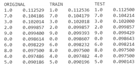
Since the metrics under study are intended to evaluate the effectiveness of binary classification, the dataset is reclassified into 2 classes – units and non-units. The proportions of data after the redistribution of classes: 11.25% of units, and 88.75% of other numbers. Before feeding the data into the algorithm, it should also be standardized so that the error function is not lengthened along a feature compared to other features. This will slow down the model convergence. To do this, the average value of the images should be subtracted from the images and divided by the standard deviation. These indicators are calculated for the entire training set, in all pixels of the images. Then the same metrics are used to standardize the test set, to ensure that the algorithm’s performance on real data is as accurate as possible, and for the state of the real data (Figure 8).
Figure 8. Dataset data visualization MNIST digits: a) before standardization; b) after standardization
To compare the performance of the algorithm and analyses the studied metrics, an experiment is conducted on another dataset – UCI ML Breast Cancer Wisconsin (Diagnostic) dataset [8]. It contains 569 vectors with 30 numerical features and corresponding class labels (0 – malignant, 1 – benign). Each of them characterizes the cell nuclei present in the breast image. Figure 9 shows a fragment of the studied dataset.
To split the training and test data, a stratified sample by class was used. The principle of division is described above when dividing the MNIST digits dataset. The division resulted in two classes, where the amount of data for each class is: Class 0 – 37%, Class 1 – 63% (where 0 is the proportion of malignant cells and 1 – benign cells). The proportions of the two classes are shown in Figures 10 and 11.
To scale the dataset, standardization by each feature was used. Two features were used to visualize the standardization (Figure 12).
For binary classification tasks, classes are divided into two parts: Positive and Negative (units and non-units, respectively). All predictions are divided into 4 parts:
1. True Positive (TP) – correct predictions of the Positive class (one is one).
2. False Positive (FP) – incorrect predictions of the Positive class (not one is one).
3. True Negative (TN) – correct predictions of the Negative class (not one is not one).
4. False Negative (FN) – incorrect predictions of the Negative class (one is not one).
Figure 9. UCI ML Breast Cancer Wisconsin (Diagnostic) dataset fragment
Figure 10. UCI ML Breast Cancer Wisconsin (Diagnostic) dataset class ratio
Figure 11. Data proportions in sample classes of the UCI ML Breast Cancer Wisconsin (Diagnostic) dataset
Figure 12. Visualization of UCI ML Breast Cancer Wisconsin (Diagnostic) dataset data: a) before standardization; b) after standardization
The classification methods were evaluated using a combination of accuracy, confusion matrices, precision, recall, F1 score, PR curves, ROC curves, PR and ROC threshold curves, and AUC. Cross-validation was utilized to create multiple train-test splits of the data and average the metrics across folds to obtain more reliable estimates. The metrics were first evaluated on the validation sets during model selection, and final performance was reported on the held-out test sets. Plotting PR and ROC curves showed the tradeoff between metrics like precision/recall and TPR/FPR at different threshold values and allowed selecting an optimal threshold. By thoroughly evaluating the methods using these varied metrics on train/validation/test splits of the data, their performance could be robustly assessed and optimized.
The class ratio in the UCI ML dataset Breast Cancer Wisconsin (Diagnostic): 11.25% of units, and 88.75% of other numbers. And if the algorithm always classifies a number as not a unit, it is almost 89% accuracy. That is, it is not suitable for evaluating datasets with different proportions of classes (5):
accuracy $=(T P+T N) /(T P+T N+F P+F N)$ (5)
Using cross-validation on 5 blocks and averaging the model estimates on them, the accuracy values were obtained – 0.988. The Confusion matrix evaluation method describes the algorithm’s work in more detail, allowing to find what mistakes the model makes [11]. It shows how many times class element A was selected as class B (Figure 13).
Figure 13. Confusion matrix for the data under study
In Figure 13, the row index of the Confusion matrix indicates the true class, and the column index indicates the predicted class. That is:
This shows that the algorithm’s performance is not as perfect as the accuracy calculations show. It is quite good at predicting class 0, but worse at predicting class 1. A confusion matrix provides a lot of information about the algorithm’s performance, but sometimes a more concise metric that is easy to graph is needed. Therefore, Precise will be used, which is the ratio of the number of correct predictions of the Positive class to the total number of predictions that the algorithm considers to be Positive. This metric indicates how often incorrect predictions occur among the predictions of the Positive class (6):
precise $=\frac{T P}{(T P+F P)}$ (6)
The calculation of precise for the covariance matrix shown in Figure 13 is (7): precise=5917/(5917+385)=0.94. But this metric is not enough, because it can be maximised if the algorithm simply learns to predict only 1 correct element of the Positive class and assigns all the others to the Negative class, i.e., precise=1/(1+0)=1. Therefore, it is necessary to have an additional evaluation that gives an understanding of how many elements of the Positive class are correctly predicted. To do this, it is necessary to use the recall metric – the proportion of Positive class images that the algorithm correctly recognised following all Positive class images (7):
recall $=\frac{T P}{(T P+F N)}$ (7)
The recall calculation for the covariance matrix shown in Figure 13 is as follows: recall=5917/(5917+221)=0.96. A recall is also called Sensitivity or True Positive Rate (TPR). Using these metrics, the algorithm can be tailored to a specific task. For example, the task is to classify sick people: sick – positive class, healthy – negative class. For this task, completeness is more important than accuracy, because if there is a healthy person among the predicted patients, it is not so bad. After all, they can be retested, but if not, all patients are classified as sick, it is an issue. Because the patient will not receive timely treatment and may infect others.
Another example is the classification of safe substances. A positive class is a safe substance, and a negative class is a hazardous substance. Accuracy is more important here because if not all hazardous substances are classified as safe, this will lead to minimal negative consequences. However, if a hazardous substance is classified as safe, the consequences can be dire [12]. The quality of the classification also depends on which class is chosen as positive and which is negative. That is, if in the example of classifying sick people, a healthy person is a positive class, and a sick person is a negative class, then the data that accurately reflects the class will be interesting, not the completeness of the class.
Another equally important metric is the Decision Threshold. It determines which class the predictions belong to. If the prediction value is higher than the threshold, it belongs to the Positive class, and if it is lower, it belongs to the Negative class. It can be interpreted as follows: if the probability that this image belongs to the Positive class is greater than the threshold, then it is assigned to the Positive class, otherwise – to the Negative class. It is inconvenient to determine the $\hat{y}$ threshold by the output of the algorithm since most predictions are either close to 0 or 1. Therefore, the threshold is estimated by the sigmoid argument (w*x). To ensure the desired ratio of precision and recall, a threshold must be selected. For this purpose, the Precision-Recall-threshold curve (PRtc) is used [13]. This graph shows precision and recalls as a function of the decision threshold. Figure 14 shows that as the threshold increases, precision increases and recall decreases, and vice versa.
Figure 14. PR threshold curve graph presentation
For a better comparison of precision and threshold, they are also plotted on a separate graph – The Precise-Recall curve (Figure 15).
Figure 15. Representation of the PR curve
The next step is to determine the threshold value that gives the best accuracy-to-completeness ratio for a given task [14]. Figure 15 shows the best classifier that achieved maximum completeness with maximum accuracy. To determine the dependence of accuracy and completeness on the decision threshold, the scalar productx*w should be calculated for a sample of images from the MNIST digits dataset. To do this, 5 images with FP and 5 with TP features should be selected (Figure 16).
Figure 16. Representation of the scalar product of a value x*w for 5 images with FP and 5 with TP features
As such, the larger the value x*w, the closer the predicted class will be to 1, and the smaller the value will be to 0. Figure 16 shows that the algorithm evaluates some values from the zero class as if they were closer to the one class, taking them for real ones. The values are sorted based on their scores (Table 2).
Table 2. Calculation of sorted labels and scores of MNIST digits dataset images
|
Tag and Rate Images |
||||||||||
|
True tag |
0 |
8 |
1 |
1 |
1 |
8 |
8 |
1 |
8 |
1 |
|
Mark |
0.26 |
0.69 |
1.021 |
2.47 |
3.87 |
4.038 |
4.54 |
5.53 |
5.66 |
6.96 |
Now, the accuracy and completeness values will depend on the threshold set. If the threshold is set to 6, then the accuracy will be maximum: precise=TP/(TP+FP)=1/(1+0)=1. However, the completeness will be low, because along with non-units, units that the algorithm cannot recognise well will be eliminated: recall=TP/(TP+FN)=1/(1+4)=0.2. At the same time, if the threshold is reduced (to 0.9), the completeness will increase, because all units will be captured in the positive class. However, the accuracy will decrease, because, among the units in the positive class, there will be non-units that the algorithm cannot distinguish from units: precise=TP/(TP+FP)=5/(5+3)=5/8=0.625 and recall=TP/(TP+FN) =5/(5+0)=1. Thus, by decreasing one value, it is necessary to increase the other and vice versa. Therefore, by changing the threshold, it is impossible to increase 2 values at the same time. To increase recall and precision at the same time, a better classifier model that will give the correct score for images of different classes can be made. Another way is to increase the amount of training data so that the model can train well, or to clean the data if it is noisy [15]. The steps to be taken for this will depend on the purpose of the study.
The next step is to apply the f1 score metric. It combines accuracy and completeness, which determines the overall assessment of data classification. The geometric mean is used for this purpose [16]. Unlike the arithmetic average, this value shows a high score when both accuracy and completeness are high. The use of this metric is useful when accuracy and completeness are of equal importance for a particular task (8):
$f 1=2 *$ precise $*$ recall $/($ precise + recall $)$ (8)
Calculating the f1 score for precision and recall, the example of calculations given above is as follows: f1=2*0.94*0.96/(0.94+0.96)=0.9498. Figure 17 shows the f1 score and mean as a function of precision and recall, both of which are equal to 0.5.
Figure 17. a) Presentation of f1 score as a function of precise with a static value of recall=0.5; b) Presentation of mean as a function of precise with a static value of recall=0.5
Figure 17 shows the f1 score and mean as a function, as the graph would look the same in the reverse. From Figure 17, the f1 score is growing more slowly than the mean function. The next metric to study is specificity. It refers to the proportion of correct predictions of the negative class to all predictions that are classified as negative class. It is also called the True Negative Rate (TNR) (9):
specifity $=T N /(T N+F N)$ (9)
Therefore, False Negative Rate (FNR) is determined by the formula (10):
$\begin{gathered}\text { False Negative Rate }(F N R)=1-\text { specifity } =F N /(F N+T N)\end{gathered}$ (10)
The calculation of the specificity and FNR for the covariance matrix shown in Figure 13 is as follows: specificity $=\frac{49477}{(49477+221)}=0.995$ and False Negative Rate (FNR)=1-specificity=1-0.995=0.005.
Receiver Operating Characteristic (ROC) is a curve similar to the PR curve, but it shows a comparison of TPR (recall) and FNR (1-specificity) on a graph. Figure 18 shows the ROC curve for the trained model in orange, and the ROC curve for the model that classifies the data with a probability of ½ for each class in the black dashed line. Figure 18 also shows that as TPR (completeness) increases, FPR also increases.
Figure 18. Representation of the ROC curve
Therefore, the ROC curve of an effective classifier should stretch as far to the left as possible to have maximum completeness at zero FPR [17]. Figure 19 shows a drop in TPR at higher threshold values. This is determined by the threshold value exceeding the scores of the units, so they fall into the non-unit class, reducing the TPR.
Figure 19. Representation of the ROC threshold curve
Figure 19 also shows a sharp decrease in the FPR as the threshold decreases. This is determined by the model generally giving lower scores to non-units than to units. If the threshold is increased sufficiently, then most non-units will fall into the non-unit class, while units will remain in the unit class (e.g., with a proxy of 0.0). The ROC curve is used when the positive class has a larger proportion of data than the negative class. Or when it is more important that the algorithm does not classify a positive class as negative. PR is used when it is more important that the algorithm does not classify a negative class as positive [18]. Drawing an analogy with the example of disease tests, then: A positive class is sick, and a negative class is healthy. In this case, the ROC curve graph will be more useful as it is more important not to classify patients as healthy. If the positive class is healthy, and the negative class is sick, then the PR curve will be more interesting. Area Under Curve (AUC) is another metric for comparing classifiers. It measures the area under the curve. The most efficient classifier will have an area under the ROC curve (ROC AUC) close to 1, and a random classifier (probability of classes is equal) will have an area under the curve of 0.5 (Figure 20).
Figure 20. Presentation of the AUC metric
It can also be compared by the area under the PR curve (PR AUC). Classifiers are compared by the area under the curve that is best suited for a particular task. Table 3 groups all the metrics presented in this study. Each metric is presented with positive and negative aspects of its application.
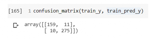
Next, the evaluation of the UCI ML Breast Cancer Wisconsin (Diagnostic) dataset classifier is described, and the decision threshold is set to achieve the desired precision/recall ratio. To begin with, the classifier is evaluated using the accuracy metric, using the cross-validation technique, and averaging the scores for all blocks [19]. As a result, the accuracy is 0.86. Since the dataset is skewed (different proportions of data in the classes), the inaccuracy matrix (built using cross-validation) should be used to better evaluate the algorithm (Figure 21).
Figure 21. Calculation of the inaccuracy matrix
The results in Figure 21 show that the algorithm makes fewer errors. It does not classify the second class as the first class (healthy as sick) because 10/(10+275)<11/(11+159). This behavior is expected since the amount of training data for the second class is larger. It is necessary to measure the precision and recall metrics using cross-validation: precision=0.91, recall=0.94. For this task, it is more important not to classify patients as healthy, i.e., high accuracy is the priority. To achieve it, the decision threshold should be changed. The results show that the positive class has a higher ratio and is more important for the algorithm not to classify the negative class as positive (sick to healthy). To do this, a PR curve should be plotted to select the best precision/recall ratio, and a PR curve with a decision threshold to select the threshold to achieve the posterior ratio (Figure 22).
Table 3. General table of the studied metrics
|
Metrics |
Advantages |
Disadvantages |
|
Accuracy |
A brief assessment that gives a general understanding of the algorithm |
Not detailed, it is not clear on which classes the algorithm works better/worse |
|
Confusion matrix |
A detailed description of the algorithm |
Sometimes a more concise assessment is more useful, for example for visualisation |
|
Precise |
A brief assessment that gives an understanding of how often the classifier assigns a negative class to a positive class |
Does not provide an understanding of the total number of elements of a positive class |
|
Recall |
A brief assessment for an understanding of the total number of elements of a positive class |
Does not give an understanding of how often the classifier assigns a negative class to a positive class |
|
f1 score |
The concise score, which combines precision and recall, gives a general understanding of the classifier’s performance and is harder to maximise than the average |
Sometimes it is necessary to ensure a certain precision/recall ratio, so the overall score is less important |
|
PR curve |
Allows to select the desired precision/recall ratio Works best when FPs are more important than FNs, or the negative class has a larger proportion than the positive class |
It does not allow to select the decision threshold to achieve the selected ratio. The classifier performs poorly when FN features are more important than FP, and when the positive class has a larger proportion than the negative class |
|
PR – threshold curve |
Allows to select the decision threshold to achieve the selected precise/recall ratio |
Sometimes it’s harder to find the right precision/recall ratio |
|
ROC curve |
Allows to select the desired TPR/FPR ratio Works best when FN features are more important than FP, or the positive class has a larger proportion than the negative class |
Does not allow to select the decision threshold to achieve the selected ratio The classifier scores worse when FP is more important than FN, and when the negative class has a larger proportion than the positive class |
|
ROC – threshold curve |
Allows to select the decision threshold to achieve the selected TPR/FPR ratio |
Sometimes it is harder to find the right TPR/FPR ratio |
|
AUC |
Provides a brief overall evaluation of the classifier’s performance, separate for PR, and ROC |
Does not describe in detail the operation of the classifier, does not give an estimate of the TPR/FPR or precise/recall ratios |
Figure 22. Presented: a) PR – decision threshold curve; b) PR curve
Figure 22b shows that to achieve approximately 97% accuracy with 85% completeness, i.e., 97% of patients will be classified as sick, but also 15% of healthy patients will be classified as sick. Therefore, the results in Figure 22a can be used to set the desired decision threshold. By setting the decision threshold to 5, an accuracy of 0.984 was achieved, with a completeness of 0.873. The threshold was set using the validation datasets obtained through cross-validation. The next step is to train the model on the full training data set. To do this, set the threshold to 5 and evaluate the accuracy and completeness. It is not possible to adjust the threshold to the test set, as the algorithm will be retrained on the test data. Therefore, the classifier’s score on the test data will not correspond to its performance on real data. After doing this, the precision is 1 and the recall is 0.916. The better result on the test data is explained by the increase in the training dataset since there is no need to allocate part of it to the validation data set [20]. The results obtained are correct for the study and confirm the need to use the above metrics for a deeper analysis of the classifier’s behavior and its impact on it. Since without their use to change the decision threshold, the algorithm will work worse for the task (precision=0.91, recall=0.94). After changing the threshold – (precision=0.984, recall=0.873).
The PR curve was selected to analyses the classifier. The precision and recall metrics were used for a detailed analysis of the classifier performance. A PR-threshold curve was constructed to select the optimal value of the decision threshold to achieve the desired precise/recall ratio for the task of classifying malignant tumors. For the task at hand, it is more important that the algorithm does not classify patients as healthy. To do this, it is necessary to select a decision threshold that will ensure maximum precision with an acceptable recall. Using the PR curve and the PR-threshold curve, a threshold of 5 is chosen, which allowed to achieve 100% accuracy with 91% completeness and an f1 score of 95.6% on the test data.
Some notable unexpected results were the high accuracy on MNIST but lower precision than recall, indicating false positive bias, and the lower optimal threshold for the cancer dataset, likely due to class imbalance. Additionally, more overfitting was observed from validation to test performance than typical. These surprising trends point to model limitations like class imbalance bias, insufficient regularization, and dataset differences.
The analysis and evaluation of classification metrics on the digit and cancer datasets demonstrates that no single metric fully captures model performance. Rather, metrics like precision, recall, ROC curves, etc. each provide unique insights that allow a deeper understanding of the tradeoffs and behavior of a model. The results highlight the importance of choosing appropriate metrics based on the use case priorities, whether that be optimizing for precision versus recall, or false positives versus false negatives. Thoughtfully evaluating models using train/validation/test splits, cross-validation, and tailored metrics provides a rigorous framework for assessing, selecting, and tuning optimal classification models for the problem at hand.
Following Santoso et al. [21], binary classification is the most challenging task in machine learning. The authors propose to use genetic programming instead of classical regression and artificial neural network. As a result of the experiment, it was noted that genetic programming has a high data processing speed, and the average accuracy is approximately 95%. Kini and Thrampoulidis [22] evaluated the classification error of gradient descent for the logistic and Gaussian mixture models. The researchers determined the dependence of the transition threshold and global minimum of the curve on the loss function, learning model, and sample size. The error of gradient descent with logistic losses undergoes a double descent, which has been proven. Moreover, the double descent depends on both the size of the model and the training epoch [23-25]. Deng et al. [26] studied the phenomenon of double descent and developed a logistic regression model based on gradient descent with logistic losses. Using Gauss’s minimum-minimum theorem, the authors characterized support vector machine solutions. Curves characterizing the classification error at different values of the phase transition threshold were obtained [27, 28]. Similar to the study [21, 22, 26], the current evaluation examined logistic regression models and accuracy metrics. However, more advanced classifiers like Santoso’s et al. [21] genetic programming achieved higher accuracy, exposing limitations of my basic methodology.
Dokeroglu et al. [29] proposed a multi-objective algorithm, Harris’ Hawks Optimisation, for solving binary classification problems. For this purpose, a new discrete perching and besieging learning operator was used. The accuracy of the prediction of the selected features was calculated using the methods of extreme learning machines, logistic regression, decision trees and support vector machines. To test the effectiveness of this algorithm, experiments were conducted on the benchmark datasets of the University of California, Irvine, and the coronavirus disease. Following the results, Harris’ Hawks Optimisation has higher accuracy than classical algorithms. Zhao et al. [30] developed a binary classification model of a quantum neural network based on an improved Grover algorithm on partial diffusion. The Younes algorithm was used to perform a quantum search using the local diffusion operator. According to experimental data, this model has a high level of accuracy [31, 32]. Adopting modern optimization and modeling methods could thus improve the author results.
The use of machine learning methods in biomedical research is discussed in Klen et al. [33]. The authors proposed an algorithm called “probabilistic contrasts”. This is a binary classifier that uses mixed and logarithmic models for decision-making [34-36]. This algorithm was compared with twelve other approaches using simulated and three real-world data sets. As it turned out, the probabilistic contrasts method demonstrated high accuracy on simulated data, but the performance on real data sets was lower. Nevertheless, the reliability of the proposed algorithm is higher compared to others. Pirouz et al. [37] applied binary classification, neural network, and regression analysis to identify confirmed COVID-19 cases. They developed a binary classification model based on a neural network with a group data mining algorithm. The input dataset included the following factors: minimum, maximum, and average air temperature, relative humidity, wind speed, and population density. The output dataset includes the number of confirmed cases of coronavirus disease within thirty days. The trend analysis was conducted in five provinces of China: Guangdong, Zhejiang, Henan, Hubei, and Hunan. The study revealed the following: the developed algorithm has a high forecasting accuracy, and this indicator was tested based on a dataset from Wuhan. The number of confirmed cases is most affected by relative humidity and maximum air temperature per day. The relative humidity of approximately 78% in the study had a positive impact on the indicators, while the maximum temperature of 15.4℃ had a negative impact.
To carry out high-quality monitoring of the population’s health, it is important to develop an effective intelligent healthcare system [38, 39]. Medical datasets play an important role in this process. Many existing datasets are unbalanced, making it difficult to train classifiers [40]. Subsequently, this leads to a decrease in reliability, accuracy, misclassification. Kumar et al. [41] evaluated the performance of logistic regression, artificial neural network, k-nearest neighbour, naive Bayes classifier, decision tree, support vector machine, and seven balancing methods on imbalanced medical datasets. The study found that there is no universal balancing method that can provide high accuracy for any dataset. For example, the k-nearest neighbour method proved to be the most suitable for recognising liver diseases. Also, the accuracy of this method in detecting coronary heart disease is 92.2%, and when using logistic regression, this value increased to 99.2%. For the diabetes dataset, the k-nearest neighbour method proved to be the most effective, with an accuracy of about 96.2%. The author’s lack of preprocessing and imbalance mitigation likely degraded my evaluation versus these leading practices.
Chicco and Jurman [42] propose to use the Matthews correlation coefficient to increase the information content and veracity when evaluating binary classifications. The study described a task consisting of two classes: n-positive and n-negative. The model predicts the class of each data sample by assigning a positive or negative label to each. At the end of the procedure, the sample falls into one of four categories: true positive, true negative, false negative, and false positive, which was also done in this article. Analyzing such a large amount of data takes a long time, so it is suggested to use statistical indicators. Using the Matthews correlation coefficient, it becomes possible to consider the imbalance of the data set and class substitution [43-45]. In this case, this criterion has demonstrated high accuracy of forecasts in all four categories [46].
The use of the Sugeno integral in the context of machine learning is highlighted in the study by Abbaszadeh and Hullermeier [47]. The authors consider a binary classification method using the Sugeno integral as an aggregation function that combines local estimates of a sample with different features into one overall estimate. This approach is suitable for learning from ordinal data [48]. An algorithm based on linear programming was developed that converts the original feature values into local estimates. To control the flexibility of the classifier and improve the retraining process, this algorithm was generalized to k-maximum capacity, where k is the parameter to be trained [49]. The study compares the Sugeno classifier with other types. Given the prediction accuracy, this algorithm is competitive. However, it has limited performance in comparison with more powerful approaches, such as the Shoke integral.
Maheshwari et al. [50] applied a variational quantum classifier for binary classification on three datasets: synthetic, public, and private. Amplitude and basis coding methods were used, which had a positive impact on the prediction speed of the datasets. The performance of the variational quantum classifier was different for the three datasets: 68.7%, 71%, and 75%, and the values of the amplitude coding of the variational quantum classifier were 67.3%, 74.5%, and 98%. The developed model was compared with the state-of-the-art models, which revealed that the model of the variational quantum classifier outperformed the state-of-the-art analogues [51-53]. Thus, this study did not consider the impact of artificial intelligence and correlation coefficients on improving the accuracy of the binary classifier. However, many existing metrics have been studied, and their advantages and disadvantages have been identified. The use of these advanced methods described in this research provided a deeper understanding of the topic.
Limitations like small dataset size, lack of model and hyperparameter optimization, class imbalance, limited feature engineering, and oversimplified simulations using only two datasets and binary classification mean the results may not fully generalize. Expanding the evaluation to larger and more diverse real-world datasets, optimized models, multi-class problems, and more complex use cases could provide more robust guidelines for rigorous classification evaluation and tuning. The limited scope means performance on real applications may differ from these initial findings.
Using the studied metrics, the performance of the binary classifier was evaluated in detail. Each of them has its advantages and disadvantages. Therefore, it is necessary to use certain metrics depending on the task and the purpose of the evaluation. The UCI ML Breast Cancer Wisconsin (Diagnostic) dataset was evaluated, and the decision threshold for achieving the required precise/recall ratio was established. These metrics were measured using cross-validation. Within this dataset, it was necessary to change the decision threshold, as well as to build a PR curve to select the most optimal precise/recall ratio, and a PR-decision threshold curve to select the threshold to achieve the desired ratio. Using these curves, a threshold of 5 was chosen, at which the accuracy reached 100% with completeness of 91%, and the f1 score was 95.6% on the test data.
This study demonstrated a rigorous framework for holistic classification model evaluation using a variety of metrics beyond basic accuracy, established guidelines for metric selection based on use case factors, showcased optimization of precision-recall tradeoffs by tuning decision thresholds, and provided practical examples of metric analysis on image and tabular datasets. The key contributions emphasize the need for confusion matrices, PR/ROC curves, cross-validation, and other techniques to thoroughly assess model limitations and lay groundwork for improving optimization, preprocessing, and tuning in future work.
This research provides guidelines for optimizing classification models on real-world tasks through robust evaluation techniques, threshold tuning to balance metric tradeoffs, and identifying areas like class imbalance to improve performance. Suggested future work involves expanding the evaluation to larger real-world datasets using advanced classifiers, implementing imbalance mitigation, optimization, feature engineering, new metrics, visualizations, and standardized frameworks. This broader benchmarking is key for developing robust and generalizable practices for optimizing, interpreting, and trusting classification models on practical applications.
The study was created within the framework of the project financed by the National Research Fund of Ukraine, registered No. 30/0103 from 01.05.2023, "Methods and means of researching markers of ageing and their influence on post-ageing effects for prolonging the working period", which is carried out at the Department of Artificial Intelligence Systems of the Institute of Computer Sciences and Information Technologies of the Lviv Polytechnic National University.
[1] Cuzzocrea, A., Leung, C.K., Soufargi, S., Olawoyin, A.M. (2022). The emerging challenges of big data lakes, and a real-life framework for representing, managing and supporting machine learning on big arctic data. In: Advances in Intelligent Networking and Collaborative Systems: The 14th International Conference on Intelligent Networking and Collaborative Systems (INCoS-2022), pp. 161-174. https://doi.org/10.1007/978-3-031-14627-5_16
[2] Sun, J., Gui, G., Sari, H., Gacanin, H., Adachi, F. (2020). Aviation data lake: Using side information to enhance future air-ground vehicle networks. IEEE Vehicular Technology Magazine, 16(1): 40-48. https://doi.org/10.1109/MVT.2020.3014598
[3] Cheng, K., Tahir, R., Eric, L.K., Li, M. (2020). An analysis of generative adversarial networks and variants for image synthesis on MNIST dataset. Multimedia Tools and Applications, 79: 13725-13752. https://doi.org/10.1007/s11042-019-08600-2
[4] Keerthi, T., Rani, E.G., Sakthimohan, M., Abhigna Reddy, G., Selvalakshmi, D., Raja Sekar, R. (2022). MNIST handwritten digit recognition using machine learning. In: 2022 2nd International Conference on Advance Computing and Innovative Technologies in Engineering (ICACITE), Greater Noida, pp. 768-772. https://doi.org/10.1109/ICACITE53722.2022.9823806
[5] Dharia, J.N., Rahman, M.A.U., Tumma, R., Ranjan, S., Reddy, M.R. (2022). Handwritten digital recognition using machine learning. International Research Journal of Engineering and Technology, 9(1): 426-430.
[6] Pei, Y., Ye, L. (2022). Cluster analysis of MNIST data set. Journal of Physics: Conference Series, 2181(1): 012035. https://doi.org/10.1088/1742-6596/2181/1/012035
[7] The MNIST database of handwritten digits. http://yann.lecun.com/exdb/mnist/, accessed on May 15, 2023.
[8] UCI Machine Learning Repository. https://goo.gl/U2Uwz2, accessed on May 15, 2023.
[9] Boyko, N., Boksho, K. (2020). Application of the Naive Bayesian classifier in work on sentimental analysis of medical data. In: IDDM’2020: 3rd International Conference on Informatics & Data-Driven Medicine. CEUR Workshop Proceedings, Växjö, pp. 1-12. https://ceur-ws.org/Vol-2753/paper16.pdf.
[10] Boyko, N., Tkachuk, N. (2020). Processing of medical different types of data using Hadoop and Java MapReduce. In: 3rd International Conference on Informatics & Data-Driven Medicine CEUR Workshop Proceedings, Växjö, pp. 1-9. https://ceur-ws.org/Vol-2753/short15.pdf.
[11] Chakure, A. (2022). Decision tree classification. https://builtin.com/data-science/classification-tree, accessed on May 16, 2023.
[12] Hyperparameter tuning with RandomizedSearchCV. 2023. https://campus.datacamp.com/courses/supervised-learning-with-scikit-learn/fine-tuning-your-model-3?ex=10, accessed on May 17, 2023.
[13] Bartley, C. (2016). Replication Data for: South African Heart Disease. https://doi.org/10.7910/DVN/76SIQD
[14] Maklin, C. (2020). XGBoost Python example. https://towardsdatascience.com/xgboost-python-example-42777d01001e.
[15] Rathi, P., Sharma, A. (2017). A review paper on prediction of diabetic retinopathy using data mining techniques. International Journal of Innovative Research in Technology, 4: 292-297.
[16] Cortes, C., Vapnik, V.N. (1995). Support-vector networks. Machine Learning, 20: 273-297. https://doi.org/10.1007/BF00994018
[17] Humphris, R.M.V. (2020). Testing algorithm fairness metrics for binary classification problems by supervised machine learning algorithms. Vrije Universiteit Amsterdam, Amsterdam.
[18] Gradient boosting machines. http://uc-r.github.io/gbm_regression, accessed on May 20, 2023.
[19] Brownlee, J. (2016). A gentle introduction to XGBoost for applied machine learning. https://machinelearningmastery.com/gentle-introduction-xgboost-applied-machine-learning.
[20] Boyko, N., Mandych B. (2020). Technologies of object recognition in space for visually impaired people. In: 3rd International Conference on Informatics & Data-Driven Medicine. CEUR Workshop Proceedings, Växjö. https://ceur-ws.org/Vol-2753/paper24.pdf.
[21] Santoso, L.W., Singh, B., Rajest, S.S., Regin, R., Kadhim, K.H. (2021). A genetic programming approach to binary classification problem. EAI Endorsed Transactions on Energy Web, 21(31): e11. http://doi.org/10.4108/eai.13-7-2018.165523
[22] Kini, G. R., Thrampoulidis, C. (2020). Analytic study of double descent in binary classification: The impact of loss. In: 2020 IEEE International Symposium on Information Theory (ISIT)., Los Angeles, pp. 2527-2532. https://doi.org/10.1109/ISIT44484.2020.9174344
[23] Bekenov, T.N., Nussupbek, Z.T., Tassybekov, Z.T., Sattinova, Z.K. (2022). Development of a model for calculating the slip coefficients of a mechanical wheeled vehicle with two steering axles. Communications - Scientific Letters of the University of Žilina, 24(3): B211-B218.
[24] Mustafin, A., Kantarbayeva, A. (2022). A model for competition of technologies for limiting resources. Bulletin of the South Ural State University, Series: Mathematical Modelling, Programming and Computer Software, 15(2): 27-42. https://doi.org/10.14529/mmp220203
[25] Mustafin, A.T. (2015). Synchronous oscillations of two populations of different species linked via interspecific interference competition. Izvestiya Vysshikh Uchebnykh Zavedeniy. Prikladnaya Nelineynaya Dinamika, 23(4): 3-23. https://doi.org/10.18500/0869-6632-2015-23-4-3-23
[26] Deng, Z., Kammoun, A., Thrampoulidis, C. (2022). A model of double descent for high-dimensional binary linear classification. Information and Inference: A Journal of the IMA, 11(2): 435-495. https://doi.org/10.1093/imaiai/iaab002
[27] Atamanyuk, I., Shebanin, V., Kondratenko, Y., Volosyuk, Y., Sheptylevskyi, O., Atamaniuk, V. (2019). Predictive control of electrical equipment reliability on the basis of the non-linear canonical model of a vector random sequence. In Proceedings of the International Conference on Modern Electrical and Energy Systems, MEES 2019, pp. 130-133. https://doi.org/10.1109/MEES.2019.8896569
[28] Babak, V.P., Babak, S.V., Eremenko, V.S., Kuts, Y.V., Myslovych M.V., Scherbak, L.M., Zaporozhets, A.O. (2021). Models of measuring signals and fields. Studies in Systems, Decision and Control, 360: 33-59.
[29] Dokeroglu, T., Deniz, A., Kiziloz, H.E. (2021). A robust multiobjective Harris’ Hawks Optimization algorithm for the binary classification problem. Knowledge-Based Systems, 227: 107219. https://doi.org/10.1016/j.knosys.2021.107219
[30] Zhao, W., Wang, Y., Qu, Y., Ma, H., Wang, S. (2022). Binary classification quantum neural network model based on optimized Grover algorithm. Entropy, 24(12): 1783. https://doi.org/10.3390/e24121783
[31] Mustafin, A. (2014). Awakened oscillations in coupled consumer-resource pairs. Journal of Applied Mathematics, 2014: 561958. https://doi.org/10.1155/2014/561958
[32] Rika, H., Aviv, I., Weitzfeld, R. (2022). Unleashing the potentials of quantum probability theory for customer experience analytics. Big Data and Cognitive Computing, 6(4): 135. https://doi.org/10.3390/bdcc6040135
[33] Klen, R., Karhunen, M., Elo, L.L. (2020). Likelihood contrasts: A machine learning algorithm for binary classification of longitudinal data. Scientific Reports, 10: 1016. https://doi.org/10.1038/s41598-020-57924-9
[34] Baizharikova, M., Tlebayeva, G., Tlebayev, M., Beksultanov, Z., Tazhiyeva, R. (2023). Development of a new innovative technological process for continuous methane fermentation in a three-stage biogas plant. Biomass Conversion and Biorefinery. https://doi.org/10.1007/s13399-023-03812-x
[35] Orazbayev, B., Dyussembina, E., Uskenbayeva, G., Shukirova, A., Orazbayeva, K. (2023). Methods for modeling and optimizing the delayed coking process in a fuzzy environment. Processes, 11(2): 450. https://doi.org/10.3390/pr11020450
[36] Bekbauov, B., Berdyshev, A., Baishemirov, Z. (2016). Numerical simulation of chemical enhanced oil recovery processes. CEUR Workshop Proceedings, 1623: 664-676.
[37] Pirouz, B., Haghshenas, S.S., Haghshenas, S.S., Piro, P. (2020). Investigating a serious challenge in the sustainable development process: Analysis of confirmed cases of COVID-19 (new type of coronavirus) through a binary classification using artificial intelligence and regression analysis. Sustainability, 12(6): 2427. https://doi.org/10.3390/su12062427
[38] Latka, D., Waligora, M., Latka, K., Miekisiak, G., Adamski, M., Kozlowska, K., Latka, M., Fojcik, K., Man, D., Olchawa, R. (2018). Virtual reality based simulators for neurosurgeons - What we have and what we hope to have in the nearest future. Advances in Intelligent Systems and Computing, 720: 1-10.
[39] Zholmagambetova, B., Mazakov, T., Jomartova, S., Izat, A., Bibalayev, O. (2020). Methods of extracting electrocardiograms from electronic signals and images in the python environment. Diagnostyka, 21(3): 95-101. https://doi.org/10.29354/diag/126398
[40] Mukasheva, A., Iliev, T., Balbayev, G. (2020). Development of the information system based on bigdata technology to support endocrinologist-doctors. In 2020 7th International Conference on Energy Efficiency and Agricultural Engineering, EE and AE 2020 – Proceedings, article number 9278971. https://doi.org/10.1109/EEAE49144.2020.9278971
[41] Kumar, V., Lalotra, G.S., Sasikala, P., Rajput, D.S., Kaluri, R., Lakshmanna, K., Shorfuzzaman, M., Alsufyani, A., Uddin, M. (2022). Addressing binary classification over class imbalanced clinical datasets using computationally intelligent techniques. Healthcare, 10(7): 1293. https://doi.org/10.3390/healthcare10071293
[42] Chicco, D., Jurman, G. (2020). The advantages of the Matthews correlation coefficient (MCC) over F1 score and accuracy in binary classification evaluation. BMC Genomics, 21: 6. https://doi.org/10.1186/s12864-019-6413-7
[43] Mussina, A., Ceccarelli, M., Balbayev, G. (2018). Neurorobotic investigation into the control of artificial eye movements. Mechanisms and Machine Science, 57: 211-221.
[44] Balbayev, G., Ceccarelli, M., Ivanov, K. (2014). An experimental test validation of a new planetary transmission. International Journal of Mechanics and Control, 15(2): 3-7.
[45] Barlybayev, A., Sabyrov, T., Sharipbay, A., Omarbekova, A. (2017). Data base processing programs with using extended base semantic hypergraph. Advances in Intelligent Systems and Computing, 569: 28-37. https://doi.org/10.1007/978-3-319-56535-4_3
[46] Soboleva, E.V., Suvorova, T.N., Bidaibekov, E.Y., Balykbayev, T.O. (2020). Designing a personalized learning model for working with technologies of creating three-dimensional images. Science for Education Today, 10(3): 108-126. https://doi.org/10.15293/2658-6762.2003.06
[47] Abbaszadeh, S., Hullermeier, E. (2020). Machine learning with the Sugeno integral: The case of binary classification. IEEE Transactions on Fuzzy Systems, 29(12): 3723-3733. https://doi.org/10.1109/TFUZZ.2020.3026144
[48] Kerimkhulle, S., Obrosova, N., Shananin, A., Azieva, G. (2022). The nonlinear model of intersectoral linkages of Kazakhstan for macroeconomic decision-making processes in sustainable supply chain management. Sustainability, 14(21): 14375. https://doi.org/10.3390/su142114375
[49] Kerimkhulle, S., Baizakov, N., Slanbekova, A., Alimova, Z., Azieva, G., Koishybayeva, M. (2022). The Kazakhstan republic economy three sectoral model inter-sectoral linkages resource assessment. Lecture Notes in Networks and Systems, 502 LNNS: 542-550.
[50] Maheshwari, D., Sierra-Sosa, D., Garcia-Zapirain, B. (2021). Variational quantum classifier for binary classification: Real vs synthetic dataset. IEEE Access, 10: 3705-3715. https://doi.org/10.1109/ACCESS.2021.3139323
[51] Mazakov, T.Z., Jomartova, S.A., Shormanov, T.S., Ziyatbekova G.Z., Amirkhanov, B.S., Kisala, P. (2020). The image processing algorithms for biometric identification by fingerprints. News of the National Academy of Sciences of the Republic of Kazakhstan, Series of Geology and Technical Sciences, 1(439): 14-22. https://doi.org/10.32014/2020.2518-170X.2
[52] Aviv, I., Barger, A., Pyatigorsky, S. (2021). Novel machine learning approach for automatic employees' soft skills assessment: group collaboration analysis case study. In 5th International Conference on Intelligent Computing in Data Sciences, ICDS 2021. Virtual, Online: Institute of Electrical and Electronics Engineers. https://doi.org/10.1109/ICDS53782.2021.9626760
[53] Benrabah, M.E., Kadri, O., Mouss, K.N., Lakhdari, A. (2022). Faulty detection system based on spc and machine learning techniques. Revue d'Intelligence Artificielle, 36(6): 969-977. https://doi.org/10.18280/ria.360619