Marvin Chandra Wijaya
© 2020 IIETA. This article is published by IIETA and is licensed under the CC BY 4.0 license (http://creativecommons.org/licenses/by/4.0/).
OPEN ACCESS
Course Timetabling is to combine the components of teachers, students, subjects, and time. The schedule consists of days on the horizontal axis and time of the clock on the vertical axis. The best first search algorithm is an algorithm to find a solution from existing nodes. Nodes can be various types of problems. In this case, the node is a two-dimensional schedule. In course timetabling there are several constraints or called heuristic functions that must be calculated. The Heuristic function consists of two parts. The first part is a constraint that must be fulfilled (Hard Constraint). There is a schedule of conflicts of the demands of the teacher cannot teach at a certain time. The second part is a constraint which is an optimization to make the search results better in heuristic value (Soft Constraint). Student schedules and teachers are worked out sequentially so students do not wait too long. Best First Search algorithm is designed in two stages. The first step is to find the first heuristic value that must be fulfilled. The second step is to find the second heuristic value. The quality of the solution obtained is between 40% -75%. The significance of this research is that dividing the Best First Search algorithm into two stages yields advantages in terms of meeting hard constraints and the time needed to process the algorithm better.
timetabling, best first search, hard constraint, soft constraint
Timetabling problems can be defined as assigning a set of class courses into a limited number of periods, subjects, teacher's time, and student's time. The complexities and the challenges of the timetabling process showed by timetabling problems arise from the fact that a large of constraints and some of which contradict with each other [1].
The timetabling problem first appeared in the artificial intelligence literature in the 1960s. Since the 1960s, it has been the subject of many researchers. The most specific basic problem is scheduling classes of courses or events (small class or large class) in such a way that no teacher or no students (or classes) are assigned to more than one course or class at the same time. This basic problem can be solved in polynomial time or exponential time by a minimize network flow algorithm. But in a real-world application, teachers can be unavailable in some time slots. Therefore, when this constraint takes place, the resulting timetabling problem is NP-complete [2].
Timetabling is important planning in the school calendar. The class timetabling process is a process for implementing an event that contains a component of the teacher, students, and subject on the time component. If a manual system is used, the problem will take longer to find a solution, especially if the number of components and rules increases.
Timetabling not only gives practical expression to the curricular philosophy of the school but timetabling also maintains and regulates the teaching and learning pulse of the school. Scheduling that is done properly ensures the delivery of quality education for students [3].
There are some aspects that must be considered to obtain a class schedule. Aspects related to scheduling that must be involved include:
Constraints in course scheduling that must be fulfilled can be guaranteed not to be violated (hard constraint) and optimization in finding the minimum waiting time for students between classes (soft constraint) is processed using the two stages of the Best First Algorithm. The objective function attempts to optimize and minimize the idle hours between the daily teaching times of all teachers and daily student class times.
University course timetabling is assigning courses and time slots and ensuring a minimum violation of soft constraints that define the quality of the timetable. The soft constraints that define differently for each institution, can make difficulty for algorithm solvers to find good solutions fast enough to be used in a practical setting [4].
The two-stage algorithm shows how to model the timetabling problem as a partial constraint satisfaction problem and gives a solver implemented with constraint handling rules that, by performing soft constraint rule and allows for making soft constraints an active process of the problem-solving process [5].
More complex constraint means more importance of the timetabling process for the educational system and highlights the multiple objectives of the task. Moreover, it makes clear that while the timetabling practice requires adopting all requirements for each institution. Every different constraint found that hold uniquely for each institution, quality is an ill-defined feature that every institution strives to achieve. For Example, at Virginia Tech, the quality of the course schedule is evaluated by the distance that the teacher or lecturer must travel from their office rooms to the classrooms. The unique time slots for class timetabling in the various categories make it possible to segregate the university-wide timetabling problem into different independent problems [6].
At Purdue University, they have to process two separate terms along with extensive experiments solving for two central and six departmental problems, individually. The problems faced by Purdue University reach 2500 classes each semester [7]. The number of classes is very large, so processing times can take a very long time. This must be anticipated in making algorithms for scheduling.
At Hannover University, Germany, the School of Economics and Management has to create the complete timetable of all courses for a term. Approximately there are 150 weekly lectures, seminars, and other events. Every class has to accommodate approximately 5 to 650 students. The teacher number approximately 100 teachers and the student number approximately 24,000 students. The decision problem is to assign many teaching groups to time slots and rooms with soft and hard constraints are met [8]. It is also necessary to pay attention to the uncertainty and dynamic environment on these constraints in each time schedule [9].
MARA University of Technology is one of the largest universities in Malaysia. MARA University of Technology has 13 branch campuses in Malaysia. Mara University of Technology offers 144 programs, delivered by 18 faculties. The dataset differs from the other institutions reported in the literature due to weekend constraints that have to be observed [10].
At Italian high schools, the timetabling problem consists of assigning class should consider for a given number of hours per week for each teacher [11]. The amount of time allocated for each student has been determined and should not be violated. The amount of time allocated has been regulated by the government, so scheduling has new hard constraints that cannot be violated.
From previous research studies, it appears that several issues exist. In the existing problems, it appears that there are important things in the constraint. The constraint consists of hard constraints and soft constraints. Both of these problems must be solved with different levels of importance. There exist various institution timetabling problems depending on the environment and the characteristics of the particular institution [12]. The institution (University or school) timetabling problem is combinatorial and there are several strict organizational and sequence-related rules that must be considered.
Combining the two types of constraints will make the problem-solving process longer and more resource consuming. It is also difficult to overcome hard constraint problems due to the existence of soft constraints.
It also needs to be considered about the existence of highly combinatorial in the search tree. The highly combinatorial search tree will make the search time increase exponentially. The repair and enhancement of existing constraints can reduce search time. The use of two algorithm stages can also divide the two possible combinatorial possibilities. This method can also reduce the search time [13].
The best first search is a search algorithm to search the most promising node chosen according to a specified function or rule. The best first search is a method that generates nodes from the previous node. The best first search selects a new node that has the smallest cost among all leaf nodes that have been raised. The best node selection is done by using a function called the f (n) evaluation function.
The best first search evaluation function can be an estimated cost from a node to the goal. The evaluation function also can be a combination of the actual cost and estimated cost. At each step of the first best search process, nodes are selected by applying an adequate heuristic function at each node selected using certain rules for generating replacement nodes. The heuristic function is a strategy to selectively search the space for a problem state, which guides the search process carried out along the path that has the greatest probability of success [14, 15].
There are several terms used in the best-first search method [16, 17]:
The start node is a term for the initial position of a search
The current node is the node that is being run in the shortest path search algorithm
A successor is the nodes that will be checked after the current node
The node is a representation of the search area
An open list is a place to store data nodes that may be accessed from the starting node or the node being run
A closed list is a place to store node data which is also a part of the shortest path that has been obtained
The goal node is the destination node
The parent is the current node of a successor.
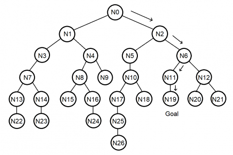
Scheduling for some tasks using the analytical hierarchy has been studied by T. Witkowski. Searching and making decisions for multi-objective scheduling has been successfully made and results in optimum scheduling [18]. At each stage, the best first search can use hyper-heuristic for the domain search. The use of some low-level heuristics makes search performance better [19]. Efficiency and optimization need to be done from design to implementation and need to be compared with other algorithms [20]. A full tree diagram as in Figure 1, is a fully open tree diagram.
Figure 1. Example of a tree search [21]
The Best First Search Algorithm requires two lists to be implemented. First is OPEN LIST which manages nodes that have been raised but have not been evaluated. Another list is CLOSE LIST which manages nodes that have been raised and evaluated. The open list and the close list contain a list of state sequences that contain a list of classes and students that have been opened or closed.
The search algorithm is as follows:
The OPEN list contains the initial state and the CLOSE LIST is still empty.
Repeat until the goal is found or until it is not in the OPEN LIST.
Take the best node in the OPEN LIST.
If the node is the same as the goal, then success.
If not, enter the node in CLOSE LIST.
Generate all successors from the node.
For each successor, do:
If the successor has never been raised, evaluate the successor, add to OPEN LIST, and record the parent.
If the successor has been raised, change the parent if the path through this parent is better than the path through the previous parent. Then update the cost for the successor and other nodes at the lower level.
Graphs that are used using non-color graphs. Color graphics are not required in solving time scheduling problems, color graphs are more widely used in Linked List-Based Exact Algorithms.
2.1 Two stages best first search
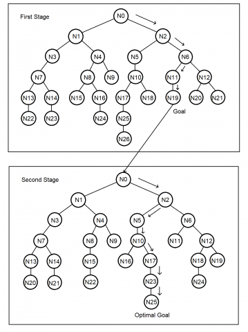
On two stages of the best-first search, the process of the best-first search algorithm is processed twice independently. Goal nodes on the first stage of the best first search algorithm is used as initial nodes on the second stage of the best-first search algorithm. Both stages use different heuristic functions. The first stage uses the hard constraints function. The second stage uses the soft constraints function. Two heuristic levels for multistage flow systems are buffers between each stage [22]. The two best first search stages produce two-stage tree diagrams as in Figure 2.
On stage two, it must be considered when opening a new node. A node that is contrary to the hard constraint is not opened. Because if it is opened it will disrupt the two-stage Best First Search Algorithm system. The use of two-stage heuristics is part of artificial intelligence that has sets of parameters that can be set to produce a combination of two optimal heuristic levels and produce the shortest time [23].
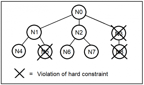
In opening a child from a node, it is important to consider the hard constraint. Nodes that violate the hard constraint will be immediately closed as in Figure 3. This makes the number of children opened smaller. This step will reduce the complexity of the course scheduling algorithm and cause a speed up timetabling process. This happens because the nodes that violate the hard constraints will be immediately removed without being added to the open list.
Figure 2. Example tree search of two Stages Best First Search
Figure 3. Example violation of hard constraints
The goal of this research is to build a weekly time table. In a week there are 5 workdays (Monday, Tuesday, Wednesday, Thursday, and Friday). Every workday there is 5 timeslots for each course class (Time slot 1, Time slot 2, Time slot 3, Time slot 4, and Time slot 5).
A node in the search tree is a two-dimensional matrix:
$N_{i}=\left[\begin{array}{lllll}S_{1,2} & S_{1,2} & S_{1,3} & S_{1,4} & S_{1,5} \\ S_{2,1} & S_{2,2} & S_{2,3} & S_{2,4} & S_{2,5} \\ S_{3,1} & S_{3,2} & S_{3,3} & S_{3,4} & S_{3,5} \\ S_{4,1} & S_{4,2} & S_{4,3} & S_{4,4} & S_{4,5} \\ S_{5,1} & S_{5,2} & S_{5,3} & S_{5,4} & S_{5,5}\end{array}\right]$ (1)
where, i is the number of nodes that are evaluated by the algorithm (i = 1, 2, 3, 4, …).
On matrix pointed in (1), columns mean days and rows mean slot- times. For every element of Ni, there is:
$S_{i, j}=\left[\begin{array}{lll}A & B & C_{i, j}\end{array}\right]$ (2)
$C_{i, j}=\{X$ who registered in subject $A \mid$ where $X$ ∈ all student list $\}$ (3)
where:
A is course/subject code.
B is the teacher code.
Ci,j is a list of students registered for A course.
The matrix pointed in (1) and (2) represents the course schedule as shown in Table 1.
Table 1. Course schedule that represented by matrix function
|
Time |
Day |
||||
|
Slot |
Monday |
Tuesday |
Wednesday |
Thursday |
Friday |
|
1 |
S1,1 |
S1,2 |
S1,3 |
S1,4 |
S1,5 |
|
2 |
S2,1 |
S2,3 |
S2,3 |
S2,4 |
S2,5 |
|
3 |
S3,1 |
S3,2 |
S3,3 |
S3,4 |
S3,5 |
|
4 |
S4,1 |
S4,2 |
S4,3 |
S4,4 |
S4,5 |
|
5 |
S5,1 |
S5,2 |
S5,3 |
S5,4 |
S5,5 |
3.1 Heuristic function
A heuristic function that is processed is a non-negative function. The standard way to build a heuristic function is to find a solution to a simpler problem, with fewer constraints. Problems with fewer constraints are often easier to solve. In many spatial problems which cost is distance and the solution are limited to going through predetermined arcs (for example, road segments), Euclidean straight lines, and more. The defined heuristic function is divided into two different heuristic functions for each stage.
3.2 First stage heuristic function
In the first stage, the heuristic formula calculation process is carried out for the teaching time of the teacher. The teacher cannot teach at any time. Every teacher has a different time slot to teach every day as pointed in (4) and (5).
$B_{i}=\left[\begin{array}{lllll}D_{1} & D_{2} & D_{3} & D_{4} & D_{5}\end{array}\right]$ (4)
$D_{i}=\{x \mid x \in x \leq 5$ and $x$ is integer $\}$ (5)
Each pair of subject schedules and teachers may not violate the teacher’s time slot. As pointed in (6) is the violation formula for one time slot and Monday.
$v_{i}=\left\{\begin{array}{ll}0, & \text { if } S_{i, 1}[A B C] \in D_{i} \\ 1, & \text { if } S_{i, 1}[A B C] \notin D_{i}\end{array}\right.$ (6)
The heuristic function for a node for this constraint is:
$f(n)=\sum_{i=1}^{5} \sum_{j=1}^{5} v_{i, j}$ (7)
Because the first stage is a hard constraint, the goal node occurs if the heuristic value is zero.
3.3 Second stage heuristic function
In the second stage, the process of calculating the heuristic formula is processed to streamline student time. Student waiting time between one course/class and another course is kept to a minimum.
The algorithm for calculating student waiting times between the two classes is:
For each class in a certain time slot student data is taken one by one.
In the next time slot is searched whether the student is registered.
If there is a student then the distance from the time slot is calculated (d = distance).
If there is no student, then look for another time slot.
The heuristic function for a node for this constraint is:
$f(n)=\sum_{i=1}^{5} \sum_{j=1}^{5} \sum_{k=1}^{n} d_{i, j, k}$ (8)
Because in the second stage is the calculation for soft constraints, the goal node is the minimum heuristic value as possible, the best value is zero but it is hard to achieve.
4.1 Set data input
The model was tested by solving an instance from a set of random data. The experiment was carried out by:
- Changing the number of teachers.
- Changing lecturer teaching hours (hard constraints)
- Changing the number of all students
- Changing the number of students registered in a lesson
This model was implemented in Personal Computer Intel® Core ™ i5-3570 CPU @ 1.40GHZ, 4 GB RAM
4.2 First stage experiments
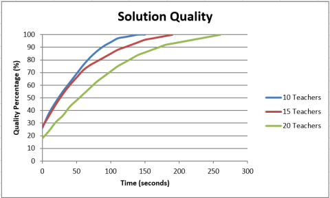
For the first stage experiment, changes were made to the number of teachers and time slots for each teacher. In one week there are 5 days X 5 time slots = 25 time slots. The number of teachers determined in the experiment was 10 teachers, 15 teachers, and 20 teachers. Each teacher is allocated 10 time slots. Experiments were carried out thirty times and the results of the experiments were averaged. The average results for each number of teachers (10, 15, and 20 teachers) are shown in Figure 4.
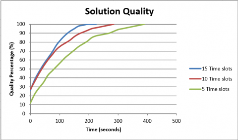
The next experiment is to change the time slot owned by each teacher. The number of teachers is was fixed, namely as many as 10 teachers. Several experiments were run for different time slots. The trial of the number of time slots held by each teacher is 5,10,15 as in Figure 5.
In this experiment, the hard constraint experiment has completed a solution worth 100%. Some of the factors obtained are the more teachers there are, the longer the processing. Similarly, the fewer time slots a teacher has, the longer the processing time.
Figure 4. Solution quality for changing the number of teachers
Figure 5. Solution quality for changing the number of time slots
4.3 Second stage experiments
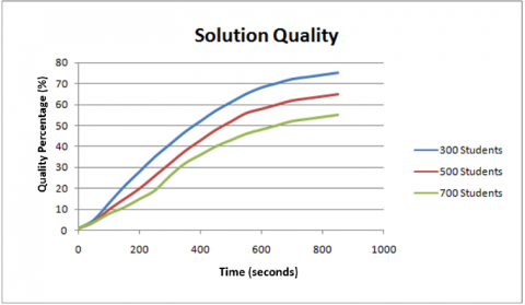
In the second stage experiment, changes were made to the number total of students. The number of students processed starts from 300, 500, and 700 students divided into several parallel classes. Meanwhile, the number of teachers and teacher time slots were fixed with data from the first stage.
Experiments were carried out thirty times and the results of the experiments were averaged. The average results for each number of students (300, 500, and 700 students) are shown in Figure 6. In this experiment, the resulting quality solution ranges from 55% to 75%. Fulfillment of soft constraints is not achieved 100%, this means that every student may have to wait between the classes that the student takes.
Figure 6. Solution quality for changing the number of total students
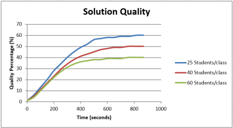
The next experiment is to change the number of students registered in a class. The number of students registered in a class starts from 25, 40, and 60 students. Meanwhile, the number of teachers and teacher time slots were determined using the first stage data.
Experiments were carried out thirty times and the results of the experiments were averaged. The average results for each number of students are shown in Figure 7.
Figure 7. Solution quality for changing the number of students registered in a class
In this experiment, the constraint experiment has not completed a solution worth 100%, the results range from 40% to 60% only. Some of the factors obtained were that the more the number of students, the smaller the percentage of the quality of the solution. Likewise, the more students in a class, the smaller the percentage of solution quality
This paper proposed a heuristic model for timetabling using two stages Best First Search Algorithm. The use of two stages serves to keep the hard constraint from being fulfilled and not modified when processing the soft constraint.
In the first stage, the heuristic function is taken from the hard constraint. The hard constraint is the availability of time or time slot from the teacher. The results of the experiment always managed to find a good solution with a relatively short time. Although the number of teachers was added, experiment results still managed to find a good solution.
In the second stage, the heuristic function is taken from the soft constraint. This soft constraint is the efficiency of student waiting time. In the second stage algorithm experiment, it was never solved with 100% quality. In an experiment with a number of students of 300 - 700 students produce solutions with a quality of 55% - 75%. In the experiment with the number of students per class that changed between 25 - 60 students per class resulted in a solution with a quality of 40% - 60%. Following the results of the second stage algorithm experiment, the time needed to process the second stage algorithm takes longer.
With the resulting solution not being able to meet all the constraints, it is necessary to make adjustments to adjust certain classes so that the resulting solution is better.
This research was supported by a Computer Engineering Department, Faculty of Engineering, Maranatha Christian University, Bandung, Indonesia. This research is fully supported by the Computer Programming Laboratory of Maranatha Christian University.
[1] Qu, R., Burke, E.K., McCollum, B., Merlot, L.T.G., Lee, S.Y. (2009). A survey of search methodologies and automated system development for examination timetabling. Journal of Scheduling, 12(1): 55-89. https://doi.org/10.1007/s10951-008-0077-5
[2] Dorneles, A.P., de Araujo, O.C.B., Buriol, L.S. (2014). A fix-and-optimize for the high school timetabling problem. Computer & Operation Research, 52: 29-38. https://doi.org/10.1016/j.cor.2014.06.023
[3] Birbas, T., Daskalaki, S., Housos, E. (2009). School timetabling for quality student and teacher schedules. Journal of Scheduling, 12(1): 177-197. https://doi.org/10.1007/s10951-008-0088-2
[4] Lindahl, M., Sorensen, M., Stidsen, T.R. (2018). A fix-and-optimize Matheuristic For University timetabling. Journal of Heuristic, 24(4): 645-665. https://doi.org/10.1007/s10732-018-9371-3
[5] Abdennadher, S., Marte, M. (2000). University course timetabling using constraint handling rules. Journal Applied Artificial Intelligence, 14(4): 311-325. https://doi.org/10.1080/088395100117016
[6] Sarin, S.C., Wang, Y., Varadarajan, A. (2010). A university-timetabling problem and its solution using Benders’ partitioning—a case study. Journal of Scheduling, 13(2): 131-141. https://doi.org/10.1007/s10951-009-0157-1
[7] Rudová, H., Müller, T., Murray, K. (2011). Complex university course timetabling. Journal of Scheduling, 14(2): 187-207. https://doi.org/10.1007/s10951-010-0171-3
[8] Schimmelpfeng, K., Helber, S. (2006). Application of a real-world university-course timetabling model solved by integer programming. OR Spectrum, 29(4): 783-803. https://doi.org/10.1007/s00291-006-0074-z
[9] Verfaillie, G., Jussien, N. (2005). Constraint solving in uncertain and dynamic environments: A survey. Constraints, 10(3): 253-281. https://doi.org/10.1007/s10601-005-2239-9
[10] Burke, E., Trick, M. (2004). A tabu search hyper-heuristic approach to the examination timetabling problem at the MARA University of Technology. Practice and Theory of Automated Timetabling V, 3616: 270-0293. https://doi.org/10.1007/11593577_16
[11] Avella, P., D’Auria, B., Salerno, S., Vasil’ev, I. (2007). A computational study of local search algorithms for Italian high-school timetabling. Journal of Heuristic, 13(6): 543-556. https://doi.org/10.1007/s10732-007-9025-3
[12] Valouxis, C., Housos, S. (2003). Constraint programming approach for school time tabling. Computer & Operation Research, 30(10): 1555-1572. https://doi.org/10.1016/S0305-0548(02)00083-7
[13] Chan, P., Weil, G. (2000). Cyclic staff scheduling using constraint logic programming. Practice and Theory of Automated Timetabling III, 3616: 155-175. https://doi.org/10.1007/3-540-44629-X_10
[14] Felner, A., Kraus, S., Korf, R.E. (2003). KBFS: K-best-first search. Annal of Mathematics and Artificial Intelligence, 39(1-2): 19-39. https://doi.org/10.1023/A:1024452529781
[15] Mencia, C., Sierra, M. R., Varela, R. (2013). An efficient hybrid search algorithm for job shop scheduling with operators. International Journal of Production Research, 51(17): 5221-5237. https://doi.org/10.1080/00207543.2013.802389
[16] Chen, Z., He, C., He, Z., Chen, M. (2018). BD-ADOPT: A hybrid DCOP algorithm with best-first and depth-first search strategies. Artificial Intelligence Review, 50(2): 161-199. https://doi.org/10.1007/s10462-017-9540-z
[17] Lam, W., Kask, K., Larrosa, J., Dechter, R. (2018). Subproblem ordering heuristics for AND/OR best-first search. Journal of Computer and System Sciences, 94: 41-64. https://doi.org/10.1016/j.jcss.2017.10.003
[18] Witkoski, R., Antczak, P., Antczak, A. (2009). Multi-objective decision making and search space for the evaluation of production process scheduling. Bulletin of The Polish Academy of Sciences Technical Sciences, 57(3): 195-208. https://doi.org/10.2478/v10175-010-0121-4
[19] Cichowicz, T., Drozdowski, M., Frankiewicz, M., Pawlak, G., Rytwinski, F., Wasilewski, J. (2012). Hyper-heuristic for cross-domain search. Bulletin of The Polish Academy of Sciences Technical Sciences, 60(4): 801-808. https://doi.org/10.2478/v10175-012-0093-7
[20] Dinu, S., Bordea, G. (2011). A new genetic approach for transport network design and optimization. Bulletin of The Polish Academy of Sciences Technical Sciences, 59(3): 263-272. https://doi.org/10.2478/v10175-011-0032-z
[21] Matsui, T., Matsuo, H. (2007). Improvement of efficiency in pseudo-tree based distributed best-first search. International Journal of Computer Science, 34(1): 71-79.
[22] Magiera, M. (2013). A relaxation heuristic for scheduling flow shops with intermediate buffers. Bulletin of The Polish Academy of Sciences Technical Sciences, 61(4): 929-942. https://doi.org/10.2478/bpasts-2013-0100
[23] Mrowczynska, B., Krol, A., Czech, P. (2019). Artificial immune system in planning deliveries in a short time. Bulletin of The Polish Academy of Sciences Technical Sciences, 67(5): 969-980. https://doi.org/10.24425/bpas.2019.12663