Akankshya Das | Sanjay Agrawal | Leena Samantaray | Rutuparna Panda* | Ajith Abraham
© 2020 IIETA. This article is published by IIETA and is licensed under the CC BY 4.0 license (http://creativecommons.org/licenses/by/4.0/).
OPEN ACCESS
The brain MR image analysis is a primary non-invasive component to detect any abnormality in the brain. It is a very important application in the field of medical image processing. For analysing brain MR images, there is a strong need to develop efficient image segmentation methods. Over the years, many image segmentation techniques have been suggested and their real life applications have also been studied. Implementation of these segmentation techniques in biomedical engineering is a major breakthrough. Intensive research works have been carried out explicitly on the analysis of human brain images and their subsequent detection of lesion cells using different segmentation methods. One of the easiest and most generally used method of segmentation is multilevel thresholding due to its precision and robustness against the other methods. To solve the problem of computational complexity for increasing threshold levels, various optimization algorithms are used for optimal multilevel thresholding. In this paper, an attempt is made to present a comprehensive review on the recent advancements in the area of brain MR image segmentation using optimal multilevel thresholding. This review is unique of its kind due to its exclusive emphasis on segmentation of brain MR image using thresholding technique only, which may not be present in the existing literature reviews. Different validation measures used for the multilevel image thresholding are discussed. A detailed comparison of the results obtained over the years is done. The merits and demerits of the methods are highlighted. This compilation aims to aid and encourage researchers to further explore the research in this direction.
biomedical imaging, brain image analysis, image processing, MRI, multilevel thresholding, optimization
The brain is the ‘master-organ’ in almost all vertebrates and invertebrates. It regulates the functioning of other organs of the body. Disorders in the brain include tumors (malignant and non-malignant), stroke (loss of cells of the brain), inflammation of brain cells and traumatic brain injury. However, brain diseases may often go undetected as there is no visible physical scar to the exterior. Clinical analysis of the abnormalities is challenging and complicated. Detection of these disorders includes brain scanning followed by image segmentation. The quality of image analysis depends on the efficiency of the segmentation method, which, in turn, is directly dependent on the image acquisition technique. Different brain scanning techniques are electroencephalography (EEG), positron emission tomography (PET), computed tomography (CT) scan, ultrasonography (USG) and magnetic resonance imaging (MRI) [1]. MRI has acquired greater popularity since it is the safest, painless, and most efficient diagnostic method. It uses no ionized radiations and obtains images of those parts that cannot be obtained through other techniques.
Image segmentation is the process of segregating different components of an image based on their intensity homogeneity, pixel values, contrast, brightness, and texture [2-4]. Based on the measure of human intervention, there are three methods of image segmentation: 1) manual, 2) semi-automatic and 3) automatic. Manual segmentation has maximum human involvement in the form of drawing the boundaries of the organ, initialization, and correction [5, 6]. It is used as a measuring standard for other segmentation techniques. However, due to its time-consuming tendency, it has clinical usage in experiments without any time constraints [7, 8]. It has got different properties like inter-rater and intra-rater variability. In inter-rater variability, different experts segment the same image differently, whereas in intra-rater variability the same image is segmented differently by the same expert at different times [9]. In semi-automatic or interactive segmentation, human involvement is limited only to initialization and correction of the segmentation method [6]. Work is done without any human interference in automatic segmentation method. Its automatic feature is facilitated by the use of model-based techniques and soft computing methods.
Medical image segmentation is challenging [10]. Here, the regions to be segmented are often non-rigid, variable in size and location and vary from person to person [11]. Brain tissue segmentation partitions the brain mainly into white matter (WM), gray matter (GM) and cerebrospinal fluid (CSF) along with its various abnormalities. There are seven objects in a brain MRI: 1) scalp, 2) bone, 3) CSF, 4) WM, 5) GM, 6) Tumor (if present), and 7) background [12]. Brain image segmentation is an integral part of brain MR image analysis. Numerous works have been done in this context. In 2015, Ivana et al. [13] presented a review article on segmentation of MR image of the human brain. They have explained various MR images, different pre-processing and post-processing steps and their validation measures. The segmentation methods have been classified into manual segmentation, intensity based, atlas based, surface based, and hybrid segmentation. A similar literature review is given in the studies [14, 15] where the authors have made a comparison of the existing methods. Anand and Kaur [14] suggest the use of high pass filtering in segmentation to obtain the accurate edges. Mathew and Babu Anto [15] have debriefed several works done in MR brain image segmentation using feature extraction and clustering methods while emphasizing on the importance of pre-processing techniques. Another work on brain tumor segmentation is given in the study [16]. This paper has made a serious review and an extensive comparison of all the existing methods using MR, PET and CT images.
In 2017, Dora et al. [17] presented a review article on brain tissue segmentation. The paper is based on extensive research of various articles on this topic in the 21st century. However, all these review papers are silent on a detailed analysis of MR brain image segmentation using thresholding approach only. These review papers have either analyzed multiple segmentation methods (thresholding, clustering etc.) or considered both medical (with or without human brain) and non-medical images (standard benchmark images line Baboon, Lena etc.) or taken into account images obtained through various scientific techniques (MRI, CT, PET). Their compositeness is their limitation. None of the works is exclusively focused on MR brain image segmentation using thresholding. Various works on thresholding of MR brain image and validation measures until this date have been discussed in details in this paper. We have focused exclusively on works done using thresholding method, as this method is the simplest, has the least computational complexity and time efficient. Moreover, it is very convenient to implement. The analysis reflects that satisfactory values are obtained in performance evaluation while using several statistical parameters. Thus, there is no compromise in the quality of the segmented image obtained in spite of the simplicity of this method. This characteristic of the segmented image has inspired us to review the method rigorously. Certain areas on this topic, which remain unexplored, have been discussed.
This review of literature is hopeful of aiding the researchers working on multilevel thresholding-based MR brain image segmentation by providing them with the required data, comparison analysis, critical review, and suggestions on the future scope of this technique.
The organization of this paper is as follows: Section 1 is the introduction. Brain MR image analysis techniques are described in Section 2. Data acquisition is discussed in Section 3. Different aspects of thresholding-based brain MR image analysis are found in the result analysis Section 4. Concluding remarks are given in Section 5.
2.1 Background
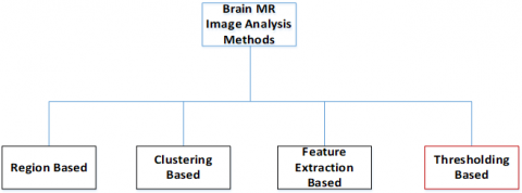
Various methods of brain MR image analysis are: 1) region-based, 2) clustering-based, 3) feature extraction and classification-based and 4) thresholding-based as presented in Figure 1. In the region-based method, a group of continuous pixels possessing homogeneous property forms a region. This similarity criterion is used for segmentation process. Different techniques used in the region-based methods are: i) contour- and shape-based method [18-22], ii) region-based level set method [23-25], iii) region growing [26-28] and iv) graph based method [29-31].
Clustering is the method of grouping tokens with high similarity. The similarity is attributed to the measurement of the Euclidean distance. The clusters thus formed, possess high intra-class similarity and low inter-class similarity. There are different types of clustering: i) k-means [32, 33], ii) fuzzy C-means [34-37] and 3) mixture models [38-40].
In several cases, the input comprises of a large amount of redundant information. Thus, the features become very large. Therefore, there is a strong need to reduce it to a sub-set consisting of only the relevant information (in the feature extraction method). This high dimensionality poses a challenge in this method. The different techniques in the feature extraction method include: Gabor filter [41-43], discrete wavelet transform (DWT) [44-47], gray level co-occurrence matrix (GLCM) and gray level run length matrix [48-51]. More elaboration on these methods is out of the scope of this review paper. Of all the methods, our paper focuses on thresholding based segmentation. Thresholding is the simplest and a very easy to implement segmentation technique for images with homogeneous objects of interest in image processing. In this method, the pixel intensity of the object under consideration is compared with one or more threshold values. Multilevel thresholding supports multiple object segmentation. These subtle properties make thresholding one of the best techniques for medical image segmentation.
Figure 1. Brain MR image analysis methods
Thresholding is a simple and efficient technique for image segmentation by comparing the pixel intensity with the threshold values. The intensity values of the pixel are classified into either object or background and the object is extracted subsequently. The process in which multiple objects can be extracted from the background is known as multilevel thresholding of an image. These methods are of two types: 1) fixed thresholding and 2) automated thresholding. In the fixed thresholding, the number of thresholds selected is fixed and pre-defined. For instance, in bi-level thresholding, the number of threshold levels selected is 1. Here, there is a single threshold value and all the pixels above this value are taken as the object while the pixels below this value are referred to as the background.
Consider an image I (x, y) where a global threshold T segments the image as:
$s(x,y)=\left\{ \begin{align} & 1,I(x,y)\ge T \\ & 0,I(x,y)<T \\ \end{align} \right.$ (1)
where, s(x,y)=1 refers to the object and s(x, y)=0 indicates the background. Similarly, in multilevel thresholding the number of threshold levels selected is greater than 1. In the automated thresholding, the number of threshold levels is variable with respect to the images being considered. This ambiguity arises due to the difficulty that lies in identifying the number of objects in the concerned image. The automatic determination of the number of threshold levels in an image is a major challenge and we did not find any relevant work that has been done in this field till date.
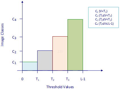
An image comprises of several components (objects) of varying intensity values. The pixel intensity of the same object has certain similarity. This concept is used to classify the pixels of an image into different classes based on the decided threshold values [see Figure 2]. The rules for a segmented output are discussed here. Let an image have intensity values from 0 to L-1. Let T1, T2 and T3 be the three threshold values used for multilevel thresholding. The image will be divided into four classes: C1 having intensity values 0 to T1, C2 having values T1+1 to T2, C3 having values T2+1 to T3 and C4 having values T3+1 to L-1.
Figure 2. Histogram representation of segmented image
There are 256 possible values or levels (L) of the pixel intensity ranging from 0 (black) to 255 (white). When the intensity of the pixel (V) lies between 0 to T1, it is assigned to class C1. The pixel intensity value in the range T1 and T2 is assigned to class C2. Class C3 is assigned, if V lies between T2 and T3. Similarly, class C4 is assigned, if V lies in between T3 and (L-1). These threshold values are then used to obtain a segmented image.
In the methods discussed above, the judicious determination of the appropriate threshold values is crucial. Various statistical parameters are used to determine the threshold values. However, their performance is affected, when these parameters get biased with any presumed information. Several research works have been conducted in order to devise methods to obtain the apt threshold values.
In 2004, Sezgin and Sankur [52] presented an elaborate survey of various image thresholding methods based on the information used. They have vividly distinguished thresholding algorithms into six categories: 1. Histogram shape information (convex haul, peak and valley, shape modelling), 2. Measurement space clustering (iterative thresholding, clustering thresholding, minimum error, fuzzy clustering), 3. Histogram entropy information (entropic, cross entropic, fuzzy entropic), 4. Image attribute information (moment preserving, edge field matching, fuzzy similarity), 5. Spatial information (co-occurrence thresholding, higher order entropy thresholding, 2-D fuzzy partitioning) and 6. Local characteristics (local variance, local contrast, Kriging method). In 1979, Otsu [53] proposed a method which aimed at maximization of the between class variance of the gray level in the histogram. It is both non-parametric and unsupervised. Initially, 1-D Otsu’s method was proposed. This method worked inefficiently with noisy images as it focused mainly on the pixel gray values without any spatial information between the pixels. It performed well only for bi-level thresholding. However, 1-D Otsu’s method is the fastest method.
Popularly used entropy-based methods are: 1) Kapur’s, 2) Shannon’s, 3) Renyi’s, 4) Cross entropy and 5) Tsallis’. Maximization of entropy i.e. probability distribution with the largest entropy gives the most accurate value. In 1980, Pun [54] proposed a method for bi-level thresholding based on the maximization of the upper bound of the total posteriori entropy. However, certain errors were detected while determining the lower bound on the posteriori entropy of the histogram. Kapur et al. [55] in 1985 have rectified this error while formulating a new algorithm. Here, the probability distribution of the entropy and the background was considered and entropy maximization was carried out. Major gap area of these methods is that their efficiency is limited to bi-level thresholding only. Another method, Shannon’s entropy [56] based segmentation is mostly based on Shannon’s information entropy where the background contains minimum information and the object carries the relevant information. Maximization of this entropy aims at maximizing the variance in inter-homogeneous region. Cross entropy is the difference in the two-probability density function where one of the distributions has the true value. Thus, it is mostly the error of the resulting value from the true distribution. A method has been devised to minimize this error.
Li et al. [57] proposed minimization of cross entropy. Minimum error thresholding [58] which aims at optimizing a constraint function based on average pixel classification error rate. This technique is applicable to both bi-level and multilevel thresholding. However, it is applicable only under the assumption that objects and pixel gray values are normally distributed. Another interesting thresholding work has been done by Portes et al. [59] by using Tsallis entropy. Generally, the Shannon entropy is an extensive entropy, which obeys Boltzmann-Gibbs-Shannon (BGS) statistics. Tsallis entropy extends it to non-extensive physical systems. It is used when non-additive information is present in the images. Another impressive innovation in this area is diagonal class entropy-based method proposed by Agrawal et al. [60]. Here the entropy is calculated along the diagonal of the gray level co-occurrence matrix and the increase in threshold level results in a reduction in computation time. Panda et al. [61] have contributed a new objective function called the evolutionary gray gradient algorithm (EGGA). This paper involves the between class variance along with the pixel average values for information loss minimization. They have made an effort to preserve the edge information along with the off diagonal pixels.
There has been an evolution of fitness functions over time. More or less works that have been proposed for multi-level thresholding-based image segmentation till date like Kapur’s entropy and 1-D Otsu function are one dimensional in nature. They have a very less number of parameters used and thus involve less computational complexity and greater speed. However, recent advancements in technology and requirement for better accuracy results have attracted researchers to the field of two-dimensional objective functions like 2-D Otsu method which have been discussed in the studies [61, 62]. Yet, the accuracy of these methods is still limited. Latest demands and progresses in image segmentation hint at a future in three-dimensional fitness functions. 3-D based methods are gaining very high popularity due to the enormous accuracy incurred while segmentation of the MR image. Multi-scale 3-D Otsu method suggested by Feng et al. [63] involves mean and median of pixel intensity information of the neighboring pixels along with the gray level of the pixel under consideration. This method exhibits greater immunity to noise and results obtained are highly stable at the cost of very high computational time.
Balanced Histogram Thresholding (BHT) is another simple objective function which divides the image into two classes i.e. background and foreground. Here, the optimal threshold value is determined by weighing the histogram followed by striking a balance between the heavier side and the lighter side [64]. Current research papers have implemented soft computing techniques with different objective functions to obtain the optimal threshold values. Earlier works indicate the contribution of Maitra and Chatterjee [65]. They have proposed the image segmentation using Kapur’s entropy. Bacterial foraging optimization (BFO) implementing ‘foraging strategy’ was used for optimization purpose. The performance of this method, called ‘BACTFOR’ has been verified using standard benchmark brain images and was compared with particle swarm optimization with linearly varying inertia weight algorithm. However, this method was inefficient due to the usage of fixed step size. The rate of convergence decreases if the step size is small while precision decreases when the step size is too high. This ambiguity can be best solved by making the step size adaptive with every iteration.
Adaptive bacteria foraging implements this technique in Kapur’s entropy and Otsu’s method [66]. Kapur’s entropy coupled with ABF resulted in high PSNR and low standard deviations while the Otsu’s method along with ABF quickly converged as compared to bacteria foraging, particle swarm optimization and genetic algorithm. A similar technique has been proposed by Sathya and Kayalvizhi [67] which focus on constantly altering the step size in order to increase the rate and precision of convergence. This paper has tried to solve multilevel thresholding problems while trying to overcome the earlier conventional works in bi-level thresholding. Genetic algorithm (GA) is a standard and one of the oldest soft computing techniques which is robust yet takes very high computation time. Hybridization of this real coded algorithm (RCGA) with Simulated Binary (SBX) cross over [68] results in better consistency and lesser standard deviation. The incorporation of SBX crossover along with polynomial mutation in this paper overcomes the gap areas in simple genetic algorithm making it more efficient.
Research work has been carried out on T2 weighted brain images were used. Threshold values were determined using maximization of Kapur’s entropy and results obtained were compared with PSO, BF, ABF, and Nelder-Mead complex. Another work on multi-level thresholding using maximization of Kapur’s entropy includes research by Priyedarsni et al. [69] which has used Social Group Optimization (SGO) method. This method resulted in modest performance evaluation values. It also focuses on extraction of tumor by using watershed segmentation. The segmented tumor region was compared with the ground truth image obtained from the BRATS MRI database. Maximization of Kapur’s entropy has also been used with Adaptive Wind Driven Optimization (AWDO) [70]. Ten benchmark brain images from the Harvard Medical School database were used for conducting the experiment and the results were compared with BFO, ABFO, PSO, GA and RCGA SBX. Analysis shows AWDO performs better than all other algorithms. This may be attributed to its adaptively changing parameters with every iteration. However, due to this feature AWDO resulted in greater convergence time than WDO. This paper has also used the Otsu’s method with AWDO and computed the results. Result comparison of this method could have been better if BRATS dataset is used. Comparison with a ground truth image should always be recommended to obtain better results for diagnosis.
In 2017, Rajnikanth et al. [71] proposed another technique for brain tissue segmentation. Here, each image undergoes tri-level thresholding using Kapur, Shannon and Tsallis entropy individually and Teaching Learning Based Optimization (TLBO) was used for the optimization purpose. After computation, it was inferred that Shannon based thresholding gave better results than its other entropy counterparts did. Another instance of use of Shannon’s entropy for tissue segmentation has been performed in [12]. Grammatical Swarm Optimization (GSO) tool has been used. This paper comprised of several processes that include denoising, intensity inhomogeneity (IIH) correction, sharpening of image and entropy maximization to obtain a segmented image. Thresholding was done on different sets of image database with and without using preprocessing steps. It was concluded that use of preprocessing steps resulted in better-segmented image, although the computation time greatly increased. Cross entropy minimization is another approach towards multilevel thresholding. This method resulted in better segmentation of colour image when used with Crow Search Algorithm (CSA) [72]. It has been implemented in general images as well as brain MR images from BrainWeb database.
Panda et al. [61] have used (EGGA) for multilevel thresholding of the brain MR image. Optimization of fitness function was done by adaptive swallow swarm algorithm (ASSO). A set of 100 images from the Harvard Medical School database have been used and their average performance parameters were calculated. The result was compared with 1-D and 2-D Otsu methods implemented with three other soft computing techniques: SSO, Coral Reef Optimization (CRO) and PSO. The intensity difference information of a 2-D histogram matrix has been proposed as a new objective function [62]. This paper has implemented Adaptive Coral Reef Optimization (ACRO) to get the optimal threshold value.
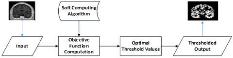
Figure 3. A generic block diagram of brain MR image analysis
Table 1. Analysis of different techniques and their implementation
|
Name of the method |
Year |
Modality |
Dataset |
Merits |
Demerits |
|
Kapur’s entropy using BFO [65] |
2008 |
Axial T2 - weighted |
Harvard Medical School |
It is less complex and easy to implement. |
Poor convergence behavior and low precision for complex optimization problems. |
|
Kapur’s entropy and Otsu’s function using Amended BFO [67] |
2011 |
Axial, T2 - weighted |
BrainWeb |
More accurate than BFO. Takes lesser convergence time. Performance is not affected by noise. |
There is still possibility of sub-optimal convergence. |
|
Kapur’s entropy and Otsu’s function using Adaptive BFO [66] |
2011 |
Axial, T2 - weighted |
BrainWeb |
Has a faster convergence. Insensitive to noise and intensity inhomogeneity. |
Chances of convergence at local optima. |
|
Kapur’s entropy using RCGA with SBX crossover [68] |
2014 |
Axial, T2 - weighted |
Harvard Medical School |
It is robust and self-adaptive in nature. It is easy to implement, performs even in noisy environment and supports multi objective optimization. |
This has greater computational complexity. |
|
Evolutionary gray gradient algorithm using Adaptive SSO in [61] |
2016 |
Axial, T2 - weighted |
Harvard Medical School |
It requires less number of parameters for tuning. There is no requirement for initialization of control parameters. Noise info is minimized due to the objective function used. |
The 1-D Otsu method is faster than this method. |
|
Kapur’s entropy using SGO [69] |
2017 |
─ |
CEREBRIX, BRAINIX and MICCAI, BRATS |
Smoother images are obtained due to skull stripping. |
There is no such remarkable difference in the image segmentation with the increase in the number of thresholds. |
|
Absolute intensity difference based technique using Adaptive CRO [62] |
2017 |
T2-weighted |
Harvard dataset, 2017 (100) |
The shape of the edges obtained was more precise. It deals with intensity inhomogeneity and gives better threshold results. |
It takes greater computation time than the 1-D Otsu method. |
|
Kapur, Shannon and Tsallis’ entropy using TLBO [71] |
2017 |
T1, T2 and Flair |
CEREBRIX, BRAINIX and BRATS |
The optimization is done without using function derivatives. |
There are chances of premature convergence at local optima. |
|
Cross entropy using CSA [72] |
2017 |
─ |
BrainWeb |
It is robust, fast, accurate, non-greedy and strikes a balance between exploration and exploitation. The number of selected threshold levels is high. The Wilcoxon rank test is done to assess the quality of results. |
Finding out the number of generations is tedious. Selection of predefined parameters is risky as incorrect selection will lead to sub-optimal convergence. |
|
Shannon’s entropy using GSO [12] |
2017 |
T2 - weighted |
Images generated by 1.5T GE MR imaging device |
It has highlighted the importance of pre- segmentation processes. This process has a broad range of application, including several other organs of the body other than the brain. |
It has very high convergence time leading to computation complexity in the case of a large dataset. The de-noising methods provide additional entropy to the image under consideration during entropy maximization. |
|
Otsu’s method and Kapur’s entropy using Adaptive WDO [70] |
2018 |
Axial T2 -weighted |
Harvard Medical School |
Due to its adaptive nature, tuning of parameters is not required. It gives better threshold values and has faster convergence as compared to other conventional methods |
Kapur-AWDO gives inaccurate results at threshold level 2 for the entire dataset. It has a greater convergence time than WDO. |
A block diagram of the brain MR image analysis using multilevel thresholding is shown in Figure 3. The brain MR image is taken as the input. Different objective functions based on various criteria are reported in the literature. These objective functions are computed using different soft computing tools. The optimal threshold values are obtained after optimizing (maximizing or minimizing) the objective function. The brain MR image is then thresholded using suitable reconstruction rules. The optimal threshold values are obtained after optimizing (maximizing or minimizing) the objective function. The brain MR image is then thresholded using suitable reconstruction rules. Table 1 presents a detailed analysis of research done in brain MR image segmentation based on multilevel thresholding using soft computing techniques.
It is found from the literature that the Otsu method [61-70] is popular due to its speed. Kapur’s entropy [65-68] is used as one of the popular techniques for multilevel thresholding due to its simplicity and accuracy. Tsalli’s entropy [71] based multilevel thresholding methods are also popular and largely accepted by the research community. Recently, many new objective functions such as Masi entropy using different optimization techniques such as Krill Herd Optimization (KHO), Harris hawks optimization (HHO) etc. are also reported in the literature for multilevel thresholding [73-92]. Researchers have also introduced fuzzy systems for dynamic parameter adaption in metaheuristics for multilevel thresholding [93-96].
It is observed that different optimization techniques are used for obtaining the optimal threshold values. Mostly, the fitness functions are based on class variance, entropy, edge magnitude and so on. It is difficult to decide the use of a particular method for a particular application. The quality of the segmentation results based on a particular method crucially depends on the choice of the parameters as well. Further, the kind of modality also plays a major concern. In summary, the reason for the choice of the method, its merits and demerits are shown in Table 1.
The performance of the segmentation technique and the quality of the output is directly dependent on the quality of the input data. MR image of the brain is the input data in this technique. This data can be acquired from real time environment (real clinical image) or can be generated artificially using a computer (synthetic image).
3.1 Real clinical images
Various real life images are obtained from several patients belonging to different gender, age groups and suffering from different brain diseases. In order to obtain a heterogeneous variety of images, maximum number of possible images must be acquired. Application of the technique on a diversity of images will validate its efficiency.
3.2 Synthetic images
These images are synthetically created using a simulator. Synthesis of the images requires predefined MR parameters.
Further modification of this image is supported based on the researcher’s requirement [17]. There is no MR scanner used and therefore generation of real images is not possible. Use of synthetic images is popular as it also has a ground truth image for comparison purposes. However, synthetic images are only a prototype of the real images and cannot take into consideration all possible factors that influence image acquisition in real time conditions.
3.3 Multimodal images
In MRI, an external magnetic field is applied to the tissues where the randomly oriented protons get arranged in a certain alignment. The protons are then excited by the application of external radio frequency (RF) energy. After some time, all the protons return to their initial position and in doing so, they emit an RF energy which is measured. This time taken for emission of RF energy is called Echo Time (TE). Repetition time (TR) is the difference in time between applications of successive pulses to the same slice. Based on the span of TR and TE various brain image modalities have been described. T1-weighted images have TR < 1000 msec and TE < 30 msec whereas T2-weighted images have TR > 2000msec and TE > 80msec [97]. Proton density (PD-weighted) images are the shorter of the two echoes employed in T2 images which use dual echo sequences. Recently, Fluid Attenuated Inversion Recovery (FLAIR) images are gaining more popularity. FLAIR is an inversion technique which results in a long inversion time that removes the signal from the CSF of the brain such that at equilibrium condition there is no net transverse magnetization of the fluid. Sometimes T1 weighted images are administered with contrast agents like gadolinium to enhance the contrast of MR images. These images are then called T1C MR Images.
Table 2. Databases used in brain tissue segmentation
|
Name of database |
Characteristics |
Download link |
|
BrainWeb |
It consists of Simulated Brain Database (SBD) generated by an MRI simulator. The images are multimodal with a variety of slice thickness, intensity, and noise levels. They are available in transversal, sagittal and coronal views. |
http://brainweb.bic.mni.mcgill.ca/brainweb
|
|
Harvard Medical School |
Numerous images are available with various conditions of the brain (normal brain, neoplastic disease, degenerative disease, and inflammatory disease). |
http://www.med.harvard.edu/aanlib/home.htm
|
|
MICCAI, BRATS |
These are clinically acquired multimodal brain images which have undergone manual segmentation. These images already have their skull stripped and intensity homogeneity removed. |
http://martinos.org/qtim/miccai2013/data.html
|
|
BRAINIX |
It is DICOM (Digital Imaging and Communication in Medicine) image sample set compressed in JPEG 2000 transfer syntax. |
https://www.osirix-viewer.com/resources/dicom-image-library |
|
CEREBRIX |
Various multimodal images are available in this DICOM file. |
https://www.osirix-viewer.com/ resources/ dicom-image-library |
Several standard databases have been decidedly declared. These are available on open source platforms for free download by researchers and teachers. These databases also contain ground truth images of various brain tissues like white matter, gray matter, and cerebrospinal fluid for comparison after segmentation process. Commonly used brain image database for research in brain tissue segmentation using thresholding are discussed in Table 2.
The efficiency of various segmentation techniques can be compared from their performance metrics. However, this comparison is challenging since all the techniques are not implemented using the same set of data (image modality and database). Some of the standard performance metrics used to compare thresholding techniques is briefly explained.
Dice similarity coefficient (DSC): Dice similarity coefficient or dicing index or Sorensen index is the quantitative spatial overlap between the ground truth image and the segmented image. It can be calculated for various tissue types since ground truth images are available for WM, GM and CSF. It can be employed in research to test the accuracy and reproducibility of the segmented image, if the ground truth images are available.
$DSC=\frac{2\left| {{I}_{s}}\cap {{I}_{g}} \right|}{\left| {{I}_{s}} \right|+\left| {{I}_{g}} \right|}$ (2)
where,
$\left|I_{s}\right|=$ cardinality of the segmented image,
$\left|I_{g}\right|=$ cardinality of ground truth image.
Its value ranges from 0 to 1. Note that 0 indicates no overlap, 1 indicates complete overlap. However, this parameter yields inaccurate results for comparison of objects with different sizes [11].
Jaccard index (JI): Jaccard index or Jaccard similarity coefficient or Tanimoto coefficient is the measure of similarity between two image sets. It is the ratio of the intersection of the segmented lesion region to ground truth lesion region. The Jaccard Index is calculated using the formula:
$JI=\frac{|{{I}_{s}}+{{I}_{g}}|}{|{{I}_{s}}|+|{{I}_{g}}|}$ (3)
The value of JI ranges from 0 to 1 where 0 indicates no segmentation and 1 denotes perfect segmentation [17]. The areas of the segmented lesion and the ground truth lesion must be of nearly the same size in order to obtain the correct results.
Similarity index (ρ): This index is often used for comparison between the segmented image and the reference image and expressed as:
$\rho =\frac{1}{C}\sum\limits_{i=1}^{C}{\frac{2|{{A}_{i}}\cap {{B}_{i}}|}{|{{A}_{i}}|+|{{B}_{i}}|}}$ (4)
Peak signal to noise ratio (PSNR): PSNR is the ratio of maximum possible signal power to the noise power affecting the quality of the signal.
$PSNR=20{{\log }_{10}}\frac{\max }{MSE}$ (5)
where, max= maximum value of the signal, MSE = mean square error. Analysis shows that we will obtain the same value of MSE when different degradations are applied to the same image [100]. Thus, PSNR is not an effective parameter to define the structural content of an image. Hore and Ziou [101] have given the relationship between PSNR and SSIM.
Inverse Difference Moment (IDM): It is the measure of local homogeneity and is also represented as HOM. Homogeneity weights values by the inverse of the contrast weight, with weights decreasing exponentially away from the diagonal [61].
Table 3. Comparison of optimal threshold values (slice #42 from the Harvard Medical School database)
|
Methods |
m |
GA |
PSO |
ABF |
Proposed |
Ref |
|
Proposed RCGA with SBX [68] |
2 |
─ |
111, 183 |
114, 184 |
114, 183 |
[68] |
|
3 |
─ |
80, 148, 178 |
74, 130, 185 |
84, 132, 187 |
||
|
4 |
─ |
81, 125, 164, 197 |
50, 100, 143, 190 |
30, 75, 127, 188 |
||
|
ProposedAWDO [70] |
2 |
111, 187 |
111, 183 |
114, 184 |
183, 256 |
[70] |
|
3 |
85, 128, 179 |
80, 148, 178 |
74, 130, 185 |
116, 186, 256 |
||
|
4 |
66, 108, 147, 188 |
81, 125, 164, 197 |
50, 100, 143, 190 |
98, 141, 189, 256 |
||
|
ProposedCHPSO [102] |
2 |
─ |
─ |
114, 184 |
112, 182 |
[102] |
|
3 |
─ |
─ |
83, 136, 187 |
82, 130, 186 |
||
|
4 |
─ |
─ |
48, 102, 144, 190 |
28, 75, 126, 186 |
||
|
1 “m” denotes the number of threshold levels; 2 “ – ” denotes data not available |
||||||
This paper analyzes efficacy of various methods, using the same data at different threshold levels, quantitatively. In general, the results obtained for bi-level thresholding may be considered inaccurate, leading to under-segmentation of the image. Thus, by increasing the threshold levels, it is possible to obtain better segmentation accuracy with much better performance evaluation metric value. However, there is also a limit to the number of threshold levels being considered, as a greater threshold level above an optimum value may result in over-segmentation. An over segmented image comprises of segmentation of the already segmented components of the image. The extracted objects from the background are again fractured into sub components in the process. This is undesirable, unnecessary and may affect the segmentation accuracy. Therefore, it is very important to limit the experiment within the optimum value. Hence, result analysis in this review concentrates only on threshold levels 2, 3, and 4. The values in bold indicate the best results obtained. Tables 3–5 give a comparison of the optimal threshold values, standard deviation, and objective function values respectively. The results are reported using the Kapur’s entropy-based method with various optimization approaches.
Table 4. Comparison of standard deviation values (slice #42 from the Harvard Medical School database)
|
Method |
m |
GA |
PSO |
ABF |
Proposed |
Ref |
|
Proposed RCGA with SBX [68] |
2 |
─ |
0.004 |
1.5000e-04 |
8.9265e-15 |
[68] |
|
3 |
─ |
0.312 |
0.019 |
7.1412e-15 |
||
|
4 |
─ |
0.539 |
0.081 |
2.0436e-04 |
||
|
Proposed AWDO [70] |
2 |
0.016 |
0.004 |
1.5000e−004 |
0.002 |
[70] |
|
3 |
0.424 |
0.312 |
0.019 |
0.006 |
||
|
4 |
0.719 |
0.539 |
0.081 |
0.020 |
||
|
Proposed CHPSO [102] |
2 |
─ |
─ |
1.5000e-4 |
8.972e-15 |
[102] |
|
3 |
─ |
─ |
0.017 |
8.972e-15 |
||
|
4 |
─ |
─ |
0.052 |
0.0003 |
Table 6 reflects the efficiency of segmentation techniques based on PSNR, SSIM, FSIM and IDM values. The values reported are the average of results obtained for 100 images from the Harvard Medical School database. This analysis reflects the best value and its degree of betterment from its competing value at threshold level 3, 4 and 5. The results clearly indicate that the same optimization technique performs differently when implemented using different objective functions. We can notice that the results obtained using the 1-D Otsu method and 2-D Otsu method are different, with the later performing better than the former. A high value of peak signal-to-noise ratio produces a better thresholded image. The table indicates that ASSO gives the best PSNR value with the 2-D Otsu method. However, the data obtained from the PSNR value using 2-D Otsu method implemented in ASSO give a surge of around 9% than that obtained using the 1-D Otsu method. This huge difference clearly reflects the better segmentation accuracy of the 2-D Otsu method. A comparison of the SSIM and FSIM values is given. The greater is the value of these parameters better is the segmentation [61]. ASSO outperforms all other techniques in all the methods computed. The table also gives a comparison of the average IDM values obtained using the 1-D Otsu method. A lesser value of IDM is desirable for better segmentation results. ASSO gives the best value, which is around 2% better than the second best competent (SSO). It may be attributed to the self-adaptive nature of the ASSO due to which very less number of parameters are required for tuning and the algorithm adaptively modifies its parameters at every iteration. When this technique is implemented using the 2-D Otsu method, we can notice a huge rise of about 14% in the results. This significant rise in value may be due to characteristic feature of the 2-D Otsu method, which takes into account gray levels of the whole image along with the spatial relationships between the pixels unlike the 1-D Otsu method, which considers the gray levels only of the image.
Table 5. Comparison of objective function values (slice #42 from the Harvard Medical School database)
|
Methods |
m |
GA |
PSO |
ABF |
Proposed |
Ref |
|
RCGA with SBX [68] |
2 |
─ |
9.256 |
9.257 |
9.258 |
[68] |
|
3 |
─ |
11.303 |
11.565 |
11.577 |
||
|
4 |
─ |
13.555 |
13.813 |
13.865 |
||
|
AWDO [70] |
2 |
9.252 |
9.256 |
9.258 |
9.100 |
[70] |
|
3 |
10.985 |
11.303 |
11.565 |
13.300 |
||
|
4 |
13.096 |
13.555 |
13.864 |
16.700 |
||
|
CHPSO [102] |
2 |
─ |
─ |
9.258 |
9.258 |
[102] |
|
3 |
─ |
─ |
11.574 |
11.578 |
||
|
4 |
─ |
─ |
13.815 |
13.865 |
Table 6. Comparison of average values of evaluation metrics (calculated over 100 slices)
|
Optimization technique |
m |
PSNR |
FSIM |
SSIM |
IDM |
||||
|
1-D Otsu |
2-D Otsu |
1-D Otsu |
2-D Otsu |
1-D Otsu |
2-D Otsu |
1-D Otsu |
2-D Otsu |
||
|
PSO [61] |
3 |
21.137 |
22.851 |
0.936 |
0.952 |
0.912 |
0.928 |
0.062 |
0.051 |
|
4 |
21.872 |
24.847 |
0.936 |
0.950 |
0.915 |
0.929 |
0.077 |
0.064 |
|
|
5 |
23.743 |
25.912 |
0.937 |
0.954 |
0.921 |
0.937 |
0.075 |
0.063 |
|
|
CRO [61] |
3 |
21.310 |
23.103 |
0.941 |
0.957 |
0.922 |
0.937 |
0.063 |
0.052 |
|
4 |
22.033 |
25.108 |
0.941 |
0.955 |
0.925 |
0.938 |
0.078 |
0.065 |
|
|
5 |
23.963 |
26.174 |
0.942 |
0.958 |
0.931 |
0.947 |
0.075 |
0.064 |
|
|
ACRO [62] |
3 |
20.390 |
22.860 |
0.941 |
0.956 |
0.922 |
0.936 |
0.056 |
0.044 |
|
4 |
21.720 |
23.830 |
0.947 |
0.959 |
0.934 |
0.946 |
0.096 |
0.047 |
|
|
5 |
22.510 |
22.511 |
0.947 |
0.963 |
0.938 |
0.954 |
0.102 |
0.058 |
|
|
SSO [61] |
3 |
21.556 |
23.336 |
0.946 |
0.962 |
0.931 |
0.947 |
0.064 |
0.052 |
|
4 |
22.296 |
25.362 |
0.946 |
0.959 |
0.934 |
0.948 |
0.077 |
0.066 |
|
|
5 |
24.226 |
26.438 |
0.947 |
0.963 |
0.940 |
0.956 |
0.076 |
0.065 |
|
|
ASSO [61] |
3 |
21.741 |
23.519 |
0.951 |
0.967 |
0.940 |
0.956 |
0.064 |
0.053 |
|
4 |
22.509 |
23.615 |
0.950 |
0.964 |
0.943 |
0.957 |
0.079 |
0.066 |
|
|
5 |
24.418 |
26.702 |
0.952 |
0.968 |
0.949 |
0.966 |
0.076 |
0.066 |
|
Figure 4. Comparison of average PSNR values
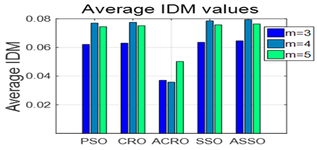
Figure 5. Comparison of average IDM values
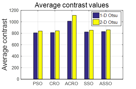
Figure 6. Comparison of average contrast values
Figure 7. Representative segmented images using various methods at threshold level 3, a) slice no 95 using EGGA, b) slice no 92 using RCGA with SBX, c) slice no 92 using AWDO
Analysis shows the improvement in these values in recent years with the adoption of faster and robust soft computing techniques. ASSO gives the highest PSNR value in 2-D Otsu method out of all the techniques used. [see Figure 4 above.]. It has the innate quality of adjusting the step size adaptively with every iteration. ASSO also outperforms other algorithms in computation of average IDM values based on the 1-D Otsu method [see Figure 5 above.]. It can also be seen that average IDM value increases with the increase in threshold level. Thus, the ASSO algorithm at threshold level 5 gives the maximum IDM value. On comparison of 1-D and 2-D Otsu methods, the later yields better result as compared to the former although the difference is small [see Figure 6 above]. The figure shows a comparison of the average contrast values of both the methods obtained at threshold level 3. It compares the values of average contrast parameters obtained using the 2-D Otsu based method. A high contrast value is desirable for better segmentation of the image. However, analysis shows that comparison results show slightly different varying result than those obtained in the parameters discussed earlier. Here, ACRO out beats ASSO by about 10%. This may be due to better efficiency of ACRO in dealing with intensity inhomogeneity.
The representative segmented images for the three methods are shown in Figure 7 above.
4.1 Challenges
Thresholding mainly focuses on the intensity values of pixels. This behavior may not guarantee the identification of contiguous pixels. Here, undesired extraneous pixels may get included along with elimination of the isolated pixels within the region. This difficulty can be overcome by using objective functions like 2-D Otsu and 3-D Otsu methods, which consider the relationship between the pixels along with pixel intensity values and result in a highly stable output. Noise removal, IIH correction and bias field correction, which may affect the MR image analysis must be taken care of. It is to be noted that Rician noise corrupts the MRI, which is image-dependent and computed from both real and imaginary images. This noise hampers quantitative estimation based on images. It should be converted into an independent Gaussian noise to eliminate the noise and apply the additive noise model. Several pre-processing and post processing steps can help in fine-tuning the segmented output. The challenge of automatically determining the number of threshold levels of an image still persists. Researchers have to manually pre-define the number of threshold levels prior to the segmentation process. This is tedious, time consuming and more of a hit and trial method. Any future scope of thresholding lies in automated thresholding and significant contribution in this area will become a major breakthrough.
4.2 Hardware implementation
Brain MR Image analysis is an important technique for detection and diagnosis of any abnormality in the brain. Acquisition of high quality (real or simulated) brain MR image is of great necessity. This is possible by using high-resolution MR instruments using superconducting magnets. Computation complexity is not an issue here as thresholding is one of the simplest methods of image segmentation. The classification of each pixel is done independent of other pixels. Thus, parallel processing is required. This greatly reduces computation time. Due to use of multiple processors, load on a single processor is reduced. Memory requirement is also low. The maximum memory that can be used is equal to the size of the image in case of storing the segmentation results [5].
4.3 Clinical usage
Brain MR Image analysis is a non-invasive exploration of the clinical details of the brain. The computational simplicity of a segmentation method determines its clinical acceptance [5]. MR image is preferred over other existing techniques for data acquisition since the images produced have a sharp contrast between fat, water, muscle, and other soft tissues. Moreover, due to the non-usage of any ionizing radiations in this process, patients are saved from exposure to such harmful radiations. There are various modalities available, which are application specific during their clinical usage. T1-weighted images are preferable for inter tissue segmentation. For intra-tissue segmentation, T2-weighted images are preferred. These images, mostly aim at detecting brain diseases associated with ageing. FLAIR images efficiently detect changes in periventricular region close to CSF along with other infarctions, multiple sclerosis, trauma, sub-arachnoid hemorrhage. Post-contrast FLAIR images detect leptomeningeal diseases. Proton density imaging. Apart from this, tissue segmentation methods are also disease specific. Therefore, it is better to use only that segmentation method which produces satisfactory results of the disease under study. Thresholding based method performs well if the tissue consists of spherical or nearly spherical.
An attempt is made to analyze the recent advances in the segmentation of the brain MR image using optimal multilevel thresholding techniques. Intriguing results on segmentation using multilevel thresholding methods are compiled in this work. Even more interesting is the comparison between various optimization methods used for multilevel thresholding. It is found that the measures like PSNR, FSIM, SSIM and IDM are well suited in evaluating a method. The performance of a methodology explicitly depends on an optimization technique. It is crucial to choose an optimization technique over the other. In this context, this study may help to enrich the knowledge on selection of an optimization technique for a particular methodology.
Methods undergoing various pre-processing (bias field correction, image registration and extraction of non-brain tissues) and post-processing stages have been observed to perform better. It is observed that the inefficiency of thresholding techniques lies in low contrast conditions in which scattered groups of pixels are formed. Therefore, use of connectivity algorithms in post processing steps will enhance the quality of the result. Most of the methods discussed in the review are manual or semi-automatic. Hence, better research in the field of segmentation using automatic approach still remains unexplored. As far as our knowledge is concerned, the maximum limit on the number of threshold levels still remains ambiguous. As stated in the literature, lesser number of threshold levels lacks distinct boundary in the segmented image, whereas higher threshold levels may result in over segmentation. Researchers need to perform segmentation on an array of threshold levels in order to obtain the appropriate number of levels. This approach is found to be tedious and time-consuming. Hence, automation of these methods to perform segmentation at the best threshold level can be the future scope in this field. Existing literature reflects very limited research using 3-D fitness functions. This area needs to be widely explored to enhance the quality of research followed by disease diagnosis. The aim of this paper is to help researchers working in this field by providing a comprehensive study on the various steps involved, data used, techniques implemented, results obtained and the future scope. It is believed that the paper may attract more readers to open the door for future research in this area.
[1] Fabijańska, A., Węgliński, T. (2014). Image processing and analysis algorithms for assessment and diagnosis of brain diseases. Computer Vision in Robotics and Industrial Applications, 513-535. https://doi.org/10.1142/9789814583725_0020
[2] Pal, N.R., Pal, S.K. (1993). A review on image segmentation techniques. Pattern Recognition, 26(9): 1277-1294. https://doi.org/10.1016/0031-3203(93)90135-J
[3] Sharma, N., Aggarwal, L.M. (2010). Automated medical image segmentation techniques. Journal of Medical Physics/Association of Medical Physicists of India, 35(1): 3-14. https://doi.org/10.4103/0971-6203.58777
[4] Gordillo, N., Montseny, E., Sobrevilla, P. (2013). State of the art survey on MRI brain tumor segmentation. Magnetic Resonance Imaging, 31(8): 1426-1438. https://doi.org/10.1016/j.mri.2013.05.002
[5] Padhani, A. (Ed.), Choyke, P. (Ed.). (2006). New Techniques in Oncologic Imaging. Boca Raton: CRC Press. Chapt. 5: 79-102. https://doi.org/10.1201/b21633
[6] Ramkumar, A., Dolz, J., Kirisli, H.A., Adebahr, S., Schimek-Jsach, T., Nestle, U., Massoptier, L., Varga, E., Stappers, P.J., Niessen, W.J., Song, Y. (2016). User interaction in semi-automatic segmentation of organs at risk: A case study in radiotherapy. Journal of Digital Imaging, 29(2): 264-277. https://doi.org/10.1007/s10278-015-9839-8
[7] Bae, K.T., Shim, H., Tao, C., Wang, J.H., Boudreau, R., Kwoh, C.K. (2009). Intra-and inter-observer reproducibility of volume measurement of knee cartilage segmented from the OAI MR image set using a novel semi-automated segmentation method. Osteoarthritis and Cartilage, 17(12): 1589-1597. https://doi.org/10.1016/j.joca.2009.06.003
[8] Gaonkar, B., Macyszyn, L., Bilello, M. (2015). Automated tumor volumetry using computer-aided image segmentation. Academic Radiology, 22(5): 653-661. https://doi.org/10.1016/j.acra.2015.01.005
[9] White, D.R., Houston, A.S., Sampson, W.F., Wilkins, G.P. (1999). Intra-and inter operator variations in region-of-interest drawing and their effect on the measurement of glomerular filtration rates. Clinical Nuclear Medicine, 24(3): 177-181. https://doi.org/10.1097/00003072-199903000-00008
[10] Balafar, M.A., Ramli, A.R., Saripan, M.I., Mashohor, S. (2010). Review of brain MRI image segmentation methods. Artificial Intelligence Review, 33(3): 261-274. https://doi.org/10.1007/s10462-010-9155-0
[11] Fasihi, M.S., Mikhael, W.B. (2016). Overview of current biomedical image segmentation methods. Computational Science and Computational Intelligence (CSCI), 2016 International Conference, Las Vegas, USA, pp. 803-808. https://doi.org/10.1109/CSCI.2016.0156
[12] Si, T., De, A., Bhattacharjee, A.K. (2015). Brain MRI segmentation for tumor detection via entropy maximization using Grammatical Swarm. International Journal of Wavelets, Multiresolution and Information Processing, 13(5): 1550039. https://doi.org/10.1142/S0219691315500393
[13] Despotović, I., Goossens, B., Philips, W. (2015). MRI segmentation of the human brain: Challenges, methods, and applications. Computational and Mathematical Methods in Medicine, 450341. https://doi.org/10.1155/2015/450341
[14] Anand, A., Kaur, H. (2016). Survey on segmentation of Brain Tumor: A review of literature. International Journal of Advanced Research in Computer and Communication Engineering, 5(1): 79-82. https://doi.org/10.17148/IJARCCE.2016.5118
[15] Mathew, A.R., Babu Anto, P. (2016). A review on MRI brain image segmentation techniques. International Journal of Innovative Research in Electrical, Electronics, Instrumentation and Control Engineering, 3(1): 100-104.
[16] Angulakshmi, M., Priya, G.G.L. (2017). Automated brain tumour segmentation techniques-A review. International Journal of Imaging Systems and Technology, 27(1): 66-77. https://doi.org/10.1002/ima.22211
[17] Dora, L., Agrawal, S., Panda, R., Abraham, A. (2017). State-of-the-art methods for brain tissue segmentation: A review. IEEE Reviews in Biomedical Engineering, 10: 235-249. https://doi.org/10.1109/RBME.2017.2715350
[18] Chan, T.F., Vese, L.A. (2001). Active contours without edges. IEEE Transactions on Image Processing, 10(2): 266-277. https://doi.org/10.1109/83.902291
[19] Latecki, L.J., Lakämper, R. (1999). Convexity rule for shape decomposition based on discrete contour evolution. Computer Vision and Image Understanding, 73(3): 441-454. https://doi.org/10.1006/cviu.1998.0738
[20] Leibe, B., Schiele, B. (2003). Analyzing appearance and contour based methods for object categorization. 2003 IEEE Computer Society Conference, Madison, USA, pp. II-409. https://doi.org/10.1109/CVPR.2003.1211497
[21] Wang, L., Chang, Y., Wang, H., Wu, Z., Pu, J., Yang, X. (2017). An active contour model based on local fitted images for image segmentation. Information Sciences, 418: 61-73. https://doi.org/10.1016/j.ins.2017.06.042
[22] Morar, A., Moldoveanu, F., Gröller, E. (2012). Image segmentation based on active contours without edges. 2012 IEEE 8th International Conference on Intelligent Computer Communication and Processing, Cluj-Napoca, România, pp. 213-220. https://doi.org/10.1109/ICCP.2012.6356188
[23] Gould, S., Gao, T., Koller, D. (2009). Region-based segmentation and object detection. 23rd Annual Conference on Neural Information Processing Systems 2009, Vancouver, Canada, pp. 655-663.
[24] Rao, T., Li, X., Zhang, H., Xu, M. (2019). Multi-level region-based convolutional neural network for image emotion classification. Neurocomputing, 14(333): 429-439. https://doi.org/10.1016/j.neucom.2018.12.053
[25] Girshick, R., Donahue, J., Darrell, T., Malik, J. (2016). Region-based convolutional networks for accurate object detection and segmentation. IEEE Transactions on Pattern Analysis and Machine Intelligence, 38(1): 142-158. https://doi.org/10.1109/TPAMI.2015.2437384
[26] Espindola, G.M., Câmara, G., Reis, I.A., Bins, L.S., Monteiro, A.M. (2006). Parameter selection for region‐growing image segmentation algorithms using spatial autocorrelation. International Journal of Remote Sensing, 27(14): 3035-3040. https://doi.org/10.1080/01431160600617194
[27] Zhang, X., Li, X., Feng, Y. (2015). A medical image segmentation algorithm based on bi-directional region growing. Optik-International Journal for Light and Electron Optics, 126(20): 2398-2404. https://doi.org/10.1016/j.ijleo.2015.06.011
[28] Mohammed, M.A., Ghani, M.K., Hamed, R.I., Abdullah, M.K., Ibrahim, D.A. (2017). Automatic segmentation and automatic seed point selection of nasopharyngeal carcinoma from microscopy images using region growing based approach. Journal of Computational Science, 1(20): 61-69. https://doi.org/10.1016/j.jocs.2017.03.009
[29] Liu, Z., Song, Y.Q., Sheng, V.S. (2019). Liver CT sequence segmentation based with improved U-Net and graph cut. Expert Systems with Applications, 126: 54-63. https://doi.org/10.1016/j.eswa.2019.01.055
[30] Zheng, Q., Li, H., Fan, B., Wu, S., Xu, J. (2018). Integrating support vector machine and graph cuts for medical image segmentation. Journal of Visual Communication and Image Representation, 55: 157-165. https://doi.org/10.1016/j.jvcir.2018.06.005
[31] Chen, X., Hu, Y., Zhang, Z., Wang, B., Zhnag, L., Shi, F., Chen, X., Jiang, X. (2019). A graph-based approach to automated EUS image layer segmentation and abnormal region detection. Neurocomputing, 336: 79-91. https://doi.org/10.1016/j.neucom.2018.03.083
[32] Katara, J., Choudhary, N. (2015). A modified version of the K-means clustering algorithm. Global Journal of Human-Social Science Research, 15(7-c).
[33] Wang, J., Su, X. (2011). An improved K-Means clustering algorithm. 2011 IEEE 3rd International Conference, Xi’an, China, pp. 44-46. https://doi.org/10.1109/ICCSN.2011.6014384
[34] Cimino, M.G., Lazzerini, B., Marcelloni, F. (2006). A novel approach to fuzzy clustering based on a dissimilarity relation extracted from data using a TS system. Pattern Recognition, 39(11): 2077-2091. https://doi.org/10.1016/j.patcog.2006.05.005
[35] Selvathi, D., Anitha, J. (2009). Effective fuzzy clustering algorithm for abnormal MR brain image segmentation. Advance Computing Conference, Patiala, India, pp. 609-614. https://doi.org/10.1109/IADCC.2009.4809081
[36] Vasuda, P., Satheesh, S. (2010). Improved fuzzy C-means algorithm for MR brain image segmentation. International Journal on Computer Science and Engineering, 2(5).
[37] Sathya, B., Manavalan, R. (2011). Image segmentation by clustering methods: Performance analysis. International Journal of Computer Applications, 29(11). https://doi.org/10.5120/3688-5127
[38] Sun, H., Yang, X., Gao, H. (2019). A spatially constrained shifted asymmetric Laplace mixture model for the grayscale image segmentation. Neurocomputing, 331: 50-57. https://doi.org/10.1016/j.neucom.2018.10.039
[39] Ji, Z., Huang, Y., Sun, Q., Cao, G. (2016). A spatially constrained generative asymmetric Gaussian mixture model for image segmentation. Journal of Visual Communication and Image Representation, 40: 611-626. https://doi.org/10.1016/j.jvcir.2016.08.001
[40] Ji, Z., Xia, Y., Sun, Q., Chen, Q., Xia, D., Feng, D.D. (2012). Fuzzy local Gaussian mixture model for brain MR image segmentation. IEEE Transactions on Information Technology in Biomedicine, 16(3): 339-347. https://doi.org/10.1109/TITB.2012.2185852
[41] Cervantes-Sanchez, F., Cruz-Aceves, I., Hernandez-Aguirre, A., Solorio-Meza, S., Cordova-Fraga, T., Aviña-Cervantes, J.G. (2018). Coronary artery segmentation in X-ray angiograms using gabor filters and differential evolution. Applied Radiation and Isotopes, 138: 18-24. https://doi.org/10.1016/j.apradiso.2017.08.007
[42] Aguirre-Ramos, H., Avina-Cervantes, J.G., Cruz-Aceves, I., Ruiz-Pinales, J., Ledesma, S. (2018). Blood vessel segmentation in retinal fundus images using Gabor filters, fractional derivatives, and expectation maximization. Applied Mathematics and Computation, 339: 568-587. https://doi.org/10.1016/j.amc.2018.07.057
[43] Dora, L., Agrawal, S., Panda, R., Abraham, A. (2017). An evolutionary single Gabor kernel based filter approach to face recognition. Engineering Applications of Artificial Intelligence, 62: 286-301. https://doi.org/10.1016/j.engappai.2017.04.011
[44] Jaffar, M.A., Mirza, A.A., Mahmud, M. (2011). MR imaging enhancement and segmentation of tumor using fuzzy curvelet. International Journal of Physical Sciences, 6(31): 7242-7246. https://doi.org/10.5897/IJPS11.418
[45] Demirel, H., Ozcinar, C., Anbarjafari, G. (2010). Satellite image contrast enhancement using discrete wavelet transform and singular value decomposition. IEEE Geoscience and Remote Sensing Letters, 7(2): 333-337. https://doi.org/10.1109/LGRS.2009.2034873
[46] Lai, C.C., Tsai, C.C. (2010). Digital image watermarking using discrete wavelet transform and singular value decomposition. IEEE Transactions on Instrumentation and Measurement, 59(11): 3060-3063. https://doi.org/10.1109/TIM.2010.2066770
[47] Mohideen, S.K., Perumal, S.A., Sathik, M.M. (2008). Image de-noising using discrete wavelet transform. International Journal of Computer Science and Network Security, 8(1): 213-216.
[48] Nabizadeh, N., Kubat, M. (2015). Brain tumors detection and segmentation in MR images: Gabor wavelet vs. statistical features. Computers & Electrical Engineering, 45: 286-301. https://doi.org/10.1016/j.compeleceng.2015.02.007
[49] Öztürk, Ş,, Akdemir, B. (2018). Application of feature extraction and classification methods for histopathological image using GLCM, LBP, LBGLCM, GLRLM and SFTA. Procedia Computer Science, 132: 40-46. https://doi.org/10.1016/j.procs.2018.05.057
[50] Pare, S., Bhandari, A.K., Kumar, A., Singh, G.K. (2017). An optimal color image multilevel thresholding technique using grey-level co-occurrence matrix. Expert Systems with Applications, 87: 335-362. https://doi.org/10.1016/j.eswa.2017.06.021
[51] Panda, R., Agrawal, S., Bhuyan, S. (2013). Edge magnitude based multilevel thresholding using Cuckoo search technique. Expert Systems with Applications, 40(18): 7617-7628. https://doi.org/10.1016/j.eswa.2013.07.060
[52] Sezgin, M., Sankur, B. (2004). Survey over image thresholding techniques and quantitative performance evaluation. Journal of Electronic Imaging,13(1): 146-166. https://doi.org/10.1117/1.1631315
[53] Otsu, N. (1979). A threshold selection method from gray-level histograms. IEEE Transactions on Systems, Man, and Cybernetics, 9(1): 62-66. https://doi.org/10.1109/TSMC.1979.4310076
[54] Pun, T. (1980). A new method for grey-level picture thresholding using the entropy of the histogram. Signal Processing, 2(3): 223-237. https://doi.org/10.1016/0165-1684(80)90020-1
[55] Kapur, J.N., Sahoo, P.K., Wong, A.K. (1985). A new method for gray-level picture thresholding using the entropy of the histogram. Computer Vision, Graphics, and Image Processing, 29(3): 273-285. https://doi.org/10.1016/0734-189X(85)90125-2
[56] El-Sayed, M.A., Hafeez, T.A. (2012). New edge detection technique based on the Shannon entropy in gray level images. arXiv:1211.2502
[57] Li, C.H., Lee, C.K. (1993). Minimum cross entropy thresholding. Pattern Recognition, 26(4): 617-625. https://doi.org/10.1016/0031-3203(93)90115-D
[58] Kittler, J., Illingworth, J. (1986). Minimum error thresholding. Pattern recognition, 19(1): 41-47. https://doi.org/10.1016/0031-3203(86)90030-0
[59] De Albuquerque, M.P., Esquef, I.A, Mello, A.G. (2004). Image thresholding using Tsallis entropy. Pattern Recognition Letters, 25(9): 1059-1065. https://doi.org/10.1016/j.patrec.2004.03.003
[60] Agrawal, S., Panda, R., Abraham, A. (2018). A novel diagonal class entropy-based multilevel image thresholding using coral reef optimization. IEEE Transactions on Systems, Man, and Cybernetics: Systems, 13(99): 1-9. https://doi.org/10.1109/TSMC.2018.2859429
[61] Panda, R., Agrawal, S., Samantaray, L., Abraham, A. (2017). An evolutionary gray gradient algorithm for multilevel thresholding of brain MR images using soft computing techniques. Applied Soft Computing, 50: 94-108. https://doi.org/10.1016/j.asoc.2016.11.011
[62] Agrawal, S., Panda, R., Samantaray, L., Abraham, A. (2017). A novel automated absolute intensity difference based technique for optimal MR brain image thresholding. Journal of King Saud University-Computer and Information Sciences. https://doi.org/10.1016/j.jksuci.2017.12.011
[63] Feng, Y., Zhao, H., Li, X., Zhang, X., Li, H. (2017). A multi-scale 3D Otsu thresholding algorithm for medical image segmentation. Digital Signal Processing, 60: 186-199. https://doi.org/10.1016/j.dsp.2016.08.003
[64] Anjos, A., Shahbazkia, H. (2008). Bi-level image thresholding-a fast method. Biosignals, 2: 70-76.
[65] Maitra, M., Chatterjee, A. (2008). A novel technique for multilevel optimal magnetic resonance brain image thresholding using bacterial foraging. Measurement, 41(10): 1124-1134. https://doi.org/10.1016/j.measurement.2008.03.002
[66] Sathya, P.D., Kayalvizhi, R. (2011). Optimal segmentation of brain MRI based on adaptive bacterial foraging algorithm. Neurocomputing, 74(14-15): 2299-2313. https://doi.org/10.1016/j.neucom.2011.03.010
[67] Sathya, P.D., Kayalvizhi, R. (2011). Amended bacterial foraging algorithm for multilevel thresholding of magnetic resonance brain images. Measurement, 44(10): 1828-1848. https://doi.org/10.1016/j.measurement.2011.09.005
[68] Manikandan, S., Ramar, K., Iruthayarajan, M.W., Srinivasagan, K.G. (2014). Multilevel thresholding for segmentation of medical brain images using real coded genetic algorithm. Measurement, 47: 558-568. https://doi.org/10.1016/j.measurement.2013.09.031
[69] Priyedarsni, P., Nandhini, B., Catherine, A.R., Sahana, K., Sundaravadivu, K. (2017). Soft-computing assisted tool to extract tumor section from brain MR images. 2017 IEEE International Conference on Power, Control, Signals and Instrumentation Engineering (ICPCSI), pp. 2776-2780. https://doi.org/10.1109/ICPCSI.2017.8392224
[70] Kotte, S., Pullakura, R.K., Injeti, S.K. (2018). Optimal multilevel thresholding selection for brain MRI image segmentation based on adaptive wind driven optimization. Measurement, 130: 340-361. https://doi.org/10.1016/j.measurement.2018.08.007
[71] Rajinikanth, V., Satapathy, S.C., Fernandes, S.L., Nachiappan, S. (2017). Entropy based segmentation of tumor from brain MR images-A study with teaching learning based optimization. Pattern Recognition Letters, 94: 87-95. https://doi.org/10.1016/j.patrec.2017.05.028
[72] Oliva, D., Hinojosa, S., Cuevas, E., Pajares, G., Avalos, O., Gálvez, J. (2017). Cross entropy based thresholding for magnetic resonance brain images using Crow Search Algorithm. Expert Systems with Applications, 79: 164-180. https://doi.org/10.1016/j.eswa.2017.02.042
[73] Resma, K.P., Nair, M.S. (2018). Multilevel thresholding for image segmentation using Krill Herd Optimization algorithm. Journal of King Saud University-Computer and Information Sciences. https://doi.org/10.1016/j.jksuci.2018.04.007
[74] Bohat, V.K., Arya, K.V. (2019). A new heuristic for multilevel thresholding of images. Expert Systems with Applications, 117: 176-203. https://doi.org/10.1016/j.eswa.2018.08.045
[75] El Aziz, M.A., Ewees, A.A., Hassanien, A.E., Mudhsh, M., Xiong, S. (2017). Multi-objective whale optimization algorithm for multilevel thresholding segmentation. Advances in Soft Computing and Machine Learning in Image Processing, 23-39.
[76] Elaziz, M.A., Ewees, A.A., Oliva, D. (2020). Hyper-heuristic method for multilevel thresholding image segmentation. Expert Systems with Applications, 146: 113201. https://doi.org/10.1016/j.eswa.2020.113201
[77] Faramarzi, A., Heidarinejad, M., Stephens, B., Mirjalili, S. (2019). Equilibrium optimizer: A novel optimization algorithm. Knowledge-Based Systems, 191: 105190. https://doi.org/10.1016/j.knosys.2019.105190
[78] Jain, M., Singh, V., Rani, A. (2018). A novel nature-inspired algorithm for optimization: Squirrel search algorithm. Swarm Evolutionary Computation, 44: 148-175. https://doi.org/10.1016/j.swevo.2018.02.013
[79] Kandhway, P., Bhandari, A.K. (2019). A water cycle algorithm-based multilevel thresholding system for color image segmentation using masi entropy. Circuits, Systems, and Signal Process, 38: 3058-3106. https://doi.org/10.1007/s00034-018-0993-3
[80] Khairuzzaman, A.K., Chaudhury, S. (2019). Masi entropy based multilevel thresholding for image segmentation. Multimed. Tools and Application, 78: 33573-33591. https://doi.org/10.1007/s11042-019-08117-8
[81] Khairuzzaman, A.K.M., Chaudhury, S. (2017). Multilevel thresholding using grey wolf optimizer for image segmentation. Expert System with Application 86: 64-76. https://doi.org/10.1016/j.eswa.2017.04.029
[82] Küçükuğurlu, B., Gedikli, E. (2020). Symbiotic organisms search algorithm for multilevel thresholding of images. Expert System with Application, 147: 113210. https://doi.org/10.1016/j.eswa.2020.113210
[83] Rodríguez, L., Castillo, O., García, M., Soria, J. (2020). Constrained real-parameter optimization using the firefly algorithm and the grey wolf optimizer. Hybrid Intelligent Systems in Control, Pattern Recognition and Medicine, 155-167. https://doi.org/10.1007/978-3-030-34135-0_11
[84] Upadhyay, P., Chhabra, J.K. (2019). Kapur’s entropy based optimal multilevel image segmentation using Crow Search Algorithm. Applied Soft Computing, 105522. https://doi.org/10.1016/j.asoc.2019.105522
[85] Wunnava, A., Naik, M.K., Panda, R., Jena, B., Abraham, A. (2020). A differential evolutionary adaptive Harris hawks optimization for two dimensional practical Masi entropy-based multilevel image thresholding. Journal of King Saud University–Computer and Information Sciences. https://doi.org/10.1016/j.jksuci.2020.05.001
[86] Wunnava, A., Kumar Naik, M., Panda, R., Jena, B., Abraham, A. (2020). An adaptive Harris hawks optimization for two dimensional grey gradient based multilevel image thresholding. Applied Soft Computing, 95: 106526. https://doi.org/10.1016/j.asoc.2020.106526
[87] Yue, X., Zhang, H. (2020). Modified hybrid bat algorithm with genetic crossover operation and smart inertia weight for multilevel image segmentation. Applied Soft Computing, 90: 106157. https://doi.org/10.1016/j.asoc.2020.106157
[88] Wunnava, A., Kumar Naik, M., Panda, R., Jena, B., Abraham, A. (2020). A novel interdependence based multilevel thresholding technique using adaptive equilibrium optimizer. Engineering Applications of Artificial Intelligence, 94: 103836. https://doi.org/10.1016/j.engappai.2020.103836
[89] Kaur, T., Saini, B.S., Gupta, S. (2018). A comparative study on Kapur's and Tsallis entropy for multilevel thresholding of MR images via particle swarm optimisation technique. International Journal of Computational Systems Engineering, 4(2-3): 156-164. https://doi.org/10.1504/IJCSYSE.2018.10012645
[90] Khairuzzaman, A.K., Chaudhury, S. (2019). Brain MR image multilevel thresholding by using particle swarm optimization, Otsu method and anisotropic diffusion. International Journal of Applied Metaheuristic Computing (IJAMC), 10(3): 91-106. https://doi.org/10.4018/IJAMC.2019070105
[91] Rajinikanth, V., Fernandes, S.L., Bhushan, B., Sunder, N.R. (2018). Segmentation and analysis of brain tumor using Tsallis entropy and regularised level set. In Proceedings of 2nd International Conference on Micro-Electronics, Electromagnetics and Telecommunications, Singapore, pp. 313-321. https://doi.org/10.1007/978-981-10-4280-5_33
[92] Kaur, T., Saini, B.S., Gupta, S. (2019). Optimization techniques for the multilevel thresholding of the medical images. Medical Data Security for Bioengineers, 166-184. https://doi.org/10.4018/978-1-5225-7952-6.ch009
[93] Castillo, O., Melin, P., Ontiveros, E., Peraza, C., Ochoa, P., Valdez, F., Soria, J. (2019). A high-speed interval type 2 fuzzy system approach for dynamic parameter adaptation in metaheuristics. Engineering Applications of Artificial Intelligence, 85: 666-680. https://doi.org/10.1016/j.engappai.2019.07.020
[94] Di, Martino, F., Sessa, S. (2020). PSO image thresholding on images compressed via fuzzy transforms. Information Science, 506: 308-324. https://doi.org/10.1016/j.ins.2019.07.088
[95] Rodríguez, L., Castillo, O., Soria, J., Melin, P., Valdez, F., Gonzalez, C.I., Martinez, G.E., Soto, J. (2017). A fuzzy hierarchical operator in the grey wolf optimizer algorithm. Applied Soft Computing, 57: 315-328. https://doi.org/10.1016/j.asoc.2017.03.048
[96] Santiago, A., Dorronsoro, B., Nebro, A.J., Durillo, J.J., Castillo, O., Fraire, H.J. (2019). A novel multi-objective evolutionary algorithm with fuzzy logic based adaptive selection of operators: FAME. Information Science, 471: 233-251. https://doi.org/10.1016/j.ins.2018.09.005
[97] Rana, R., Singh, P. (2015). Brain tumor detection through MR images: A review of literature. IOSR Journal of Computer Engineering, 17(5): 7-18.
[98] Wang, Z., Bovik, A.C., Sheikh, H.R., Simoncelli, E.P. (2004). Image quality assessment: From error visibility to structural similarity. IEEE Transactions on Image Processing, 13(4): 600-612. https://doi.org/10.1109/TIP.2003.819861
[99] Zhang, L., Zhang, L., Mou, X., Zhang, D. (2011). FSIM: A feature similarity index for image quality assessment. IEEE Transactions on Image Processing, 20(8): 2378-2386. https://doi.org/10.1109/TIP.2011.2109730
[100] Wang, Z., Bovik, A.C. (2009). Mean squared error: Love it or leave it? A new look at signal fidelity measures. IEEE Signal Processing Magazine, 26(1): 98-117. https://doi.org/10.1109/MSP.2008.930649
[101] Hore, A., Ziou, D. (2010). Image quality metrics: PSNR vs. SSIM. 20th International Conference on Pattern Recognition, Istanbul, Turkey, pp. 2366-2369. https://doi.org/10.1109/ICPR.2010.579
[102] Mozaffari, M.H., Lee, W.S. (2016). Multilevel thresholding segmentation of T2 weighted brain MRI images using convergent heterogeneous particle swarm optimization. arXiv:1605.04806.