Tingmei Wang | Yanyan Chen*
OPEN ACCESS
In recent year, the tensor theory has been frequently incorporated to machine learning, because of the various advantages of tensor-based machine learning over vector-based machining learning: the ability to preserve the spatiotemporal information, allowing full utilization of the data, and the suitability for solving high-dimensional problems with a small sample size. Considering the suitability of tensor algorithm for classical high-dimensional, small-sample problems, this paper probes into the nonlinear classification problem with tensor representation, and designs a tensor-based nonlinear classification algorithm, namely, the kernel-based STM (KSTM). The maximum margin principle was adopted for the classification by the KSTM: the two types of samples are separated by the decision hyperplane as far as possible in the tensor space. Through numerical experiments, it is proved that the KSTM achieved better classification accuracy than the linear method, especially for the high-dimensional problem with a small sample size.
tensor representation, nonlinear classification, support tensor machine (STM), image classification
Machine learning is a research hotspot in recent years. Data representation is an important problem in machine learning. The data from different sources should be expressed in a form that facilitates the application of machine learning techniques. Traditionally, the data are inputted as vectors for machine learning. In real-world scenarios, however, it is more accurate to represent data in tensor form. As a result, the tensor representation of data has become a new research direction in the field of data mining and machine learning [1-5]. Recent years has seen a growing attention being paid to tensor representation and its application in fields like image classification, face recognition, scene classification and bioinformatics [6-15].
In 2006, Cai et al. [16] proposed the support tensor machine (STM), a novel machine learning method based on tensor data. Since then, great progress has been made in the theories and learning models that solve machine learning problems based on tensor data. Compared with vector-based machine learning, the tensor-based machine learning has two unique advantages: the ability to preserve the spatiotemporal information, allowing full utilization of the data, and the suitability for solving high-dimensional problems with a small sample size. Therefore, the tensor-based machining learning can be applied well in classical high-dimensional, small-sample problems like face recognition and image classification.
Considering the nonlinearity of many real-world data, many scholars have adopted kernel methods for tensor representation. For example, Signoretto et al. [17] elaborated on a possible framework that extends the flexibility of tensor-based models with kernel-based techniques, which provides a constructive definition of the infinite dimensional tensor feature space. He et al. [18] developed a brand-new design of structure-maintaining kernels for supervised tensor learning. If the order of tensors is specified, tensor representation can be achieved by some very simple and convenient kernel methods, namely, the matrix kernel function of second-order tensor [19-22] and the K3rd kernel function for third-order tensor [23, 24].
This paper probes into the nonlinear classification problem with tensor representation, and designs a tensor-based nonlinear classification algorithm, namely, the kernel-based STM (KSTM). Since images can naturally be represented by tensor data [25-28], the proposed KSTM was applied to solve image classification problems. Through numerical experiments, it is proved that the KSTM achieved better classification accuracy than the linear method, especially for the high-dimensional problem with a small sample size.
In 2006, Cai et al. [16] extended the support vector machine (SVM) to the tensor space model under the framework of supervised tensor learning (STL). In the tensor space, the linear discriminant function can be expressed as:
$f(\mathbf{X})=\mathbf{u}^{T} \mathbf{X} \mathbf{v}+b, \mathbf{u} \in R^{n_{1}}, \mathbf{v} \in R^{n_{2}}$ (1)
The maximum margin principle is introduced to the classification process: the two types of samples are separated by the decision hyperplane as far as possible in the tensor space. Then, the corresponding optimization problem can be defined as:
$\min _{\boldsymbol{u}, \boldsymbol{v}, \boldsymbol{b}, \boldsymbol{\xi}} \frac{1}{2}\left\|\mathbf{u} \mathbf{v}^{T}\right\|^{2}+C \sum_{i=1}^{m} \xi_{i}$
s.t.$y_{i}\left(\mathbf{u}^{T} \mathbf{X}_{i} \mathbf{v}+b\right) \geq 1-\xi_{i}$ (2)
$\xi_{i} \geq 0, i=1, \dots, m$
By introducing positive Lagrangian multipliers $\alpha_{i}, \beta_{i} \geq 0$, i=1,…,m, the Lagrangian function of optimization problem (2) can be written as:
$L(\mathbf{u}, \mathbf{v}, b, \xi, \alpha, \beta)=\frac{1}{2}\left\|\mathbf{u} \mathbf{v}^{T}\right\|^{2}+C \sum_{i} \xi_{i}$$-\sum_{i} \alpha_{i} y_{i}\left(\mathbf{u}^{T} \mathbf{X}_{i} \mathbf{v}+b-1+\xi_{i}\right)-\sum_{i} \beta_{i} \xi_{i}$ (3)
Under the Karush–Kuhn–Tucker (KKT) conditions, the partial derivatives of L with respect to $\mathbf{u}, \mathbf{v}, b, \xi_{i}$, are set to zero. Then, we have:
$\mathbf{u}=\frac{\sum_{i} \alpha_{i} y_{i} \mathbf{x}_{i} \mathbf{v}}{\mathbf{v}^{T} \mathbf{v}}$ (4)
$\mathbf{v}=\frac{\sum_{i} \alpha_{i} y_{i} \mathbf{u}^{T} \mathbf{x}_{i}}{\mathbf{u}^{T} \mathbf{u}}$ (5)
$\sum_{i} \alpha_{i} y_{i}=0$ (6)
$C-\alpha_{i}-\beta_{i}=0, i=1, \ldots, m$ (7)
Formulas (4) and (5) show that u and v are dependent on each other, and cannot be solved independently. Therefore, Cai et al. [16] developed an alternative projection algorithm, providing a simple and effective method to solve this optimization problem.
Let u be a constant, $\mu_{1}=\|\mathbf{u}\|^{2}$ and $\mathbf{x}_{i}=\mathbf{X}_{i}^{T} \mathbf{u}$. Then, formulas (2) can be transformed into:
$\min _{v, b, \xi} \frac{1}{2} \mu_{1}\|\mathbf{v}\|^{2}+C \sum_{i=1}^{m} \xi_{i}$
s.t. $y_{i}\left(\mathbf{v}^{T} \mathbf{x}_{\mathbf{i}}+b\right) \geq 1-\xi_{i}$ (8)
$\xi_{i} \geq 0, i=1, \dots, m$
Formula (8) is obviously a standard SVM optimization problem. Thus, the SVM algorithm is introduced to solve the problem.
Similarly, once v is calculated, it is assumed that $\mu_{2}=\|\mathbf{v}\|^{2}$ and $\tilde{\mathbf{x}}_{i}=\mathbf{X}_{i} \mathbf{v}$. Then, u can be solved through the following optimization problem:
$\min _{\mathbf{u}, b, \xi} \frac{1}{2} \mu_{2}\|\mathbf{u}\|^{2}+C \sum_{i=1}^{m} \xi_{i}$
s.t. $y_{i}\left(\mathbf{u}^{T} \tilde{\mathbf{x}}_{i}+b\right) \geq 1-\xi_{i}$ (9)
$\xi_{i} \geq 0, i=1, \dots, m$
In this way, both v and u can be obtained by iteratively solving the optimization problems (8) and (9).
Let $\left\{\mathbf{X}_{i}, y_{i}\right\}$, i=1,…,m be a set of training samples, where $\mathbf{x}_{i} \in \mathbb{R}^{\mathrm{n}_{1}} \otimes \mathbb{R}^{\mathrm{n}_{2}}$ is a sample (data point) in a 2nd order tensor space ($\mathbb{R}^{{n}_{1}}$ and $\mathbb{R}^{{n}_{2}}$ are two vector spaces), and $y_{i} \in\{-1,1\}$ is the label of $\mathbf{X}_{i}$. The KSTM mainly aims to find a decision hyperplane by mapping the tensor data into a high-dimensional tensor feature space, such that the data points can be separated by the maximum margin from each class. Hence, the KSTM can be described as the following optimal quadratic programming problem:
$\min _{\boldsymbol{u}, \boldsymbol{v}, \boldsymbol{b}, \boldsymbol{\xi}} \frac{1}{2}\left\|\mathbf{u} \mathbf{v}^{T}\right\|^{2}+C \sum_{i=1}^{m} \xi_{i}$
s.t. $y_{i}\left(\mathbf{u}^{T} \Phi\left(\mathbf{X}_{i}\right) \mathbf{v}+b\right) \geq 1-\xi_{i}$ (10)
$\xi_{i} \geq 0, i=1, \dots, m$
Meanwhile, the decision function of a nonlinear classifier in the tensor space can be established as:
$f(\mathbf{X})=\operatorname{sgn}\left(\left(\mathbf{u v}^{T} \cdot \Phi(\mathbf{X})\right)+b\right) \quad \mathbf{u} \in \mathbb{R}^{n_{1}}, \mathbf{v} \in \mathbb{R}^{n_{2}}$ (11)
where, $\Phi$ is the function that maps the data from the original tensor space to a tensor feature space.
According to Gao’s kernel function for tensor representation [20], a nonlinear mapping function $\Phi\left(\mathbf{X}_{\mathbf{i}}\right)$ can be adopted to map $\mathbf{X}_{\mathbf{i}}$ into a high-dimensional tensor feature space:
$\Phi\left(\mathbf{X}_{i}\right)=\left[\begin{array}{c}{\varphi\left(z_{i 1}\right)} \\ {\varphi\left(z_{i 2}\right)} \\ {\vdots} \\ {\varphi\left(z_{i n_{1}}\right)}\end{array}\right]$ (12)
where, ${z}_{i p}$ is the p-th row of $\mathbf{X}_{i}$. Thus, the new kernel function for tensors can be constructed as:
$K\left(\mathbf{X}_{i}, \mathbf{X}_{j}\right)=\Phi\left(\mathbf{X}_{i}\right) \Phi\left(\mathbf{X}_{j}\right)^{T}=\left[\begin{array}{c}{\varphi\left(z_{i 1}\right)} \\ {\varphi\left(z_{i 2}\right)} \\ {\vdots} \\ {\varphi\left(z_{i n_{1}}\right)}\end{array}\right]\left[\begin{array}{c}{\varphi\left(z_{j 1}\right)} \\ {\varphi\left(z_{j 2}\right)} \\ {\vdots} \\ {\varphi\left(z_{j n_{1}}\right)}\end{array}\right]^{T}$$=\left(\begin{array}{ccc}{\varphi\left(z_{i 1}\right) \varphi\left(z_{j 1}\right)^{T}} & {\cdots} & {\varphi\left(z_{i 1}\right) \varphi\left(z_{j n_{1}}\right)^{T}} \\ {\vdots} & {\ddots} & {\vdots} \\ {\varphi\left(z_{i n_{1}}\right) \varphi\left(z_{j 1}\right)^{T}} & {\cdots} & {\varphi\left(z_{i n_{1}}\right) \varphi\left(z_{j n_{1}}\right)^{T}}\end{array}\right)$ (13)
For example, if Gaussian kernel function is employed, the ij-th element of the kernel matrix can be expressed as:
$\varphi\left(z_{i p_{1}}\right) \varphi\left(z_{j p_{1}}\right)^{T}=e^{\frac{\left\|z_{i p_{1}}-z_{i p_{2}}\right\|^{2}}{2 \sigma^{2}}}$ (14)
Obviously, the kernel function for tensors differs from that for vectors. The result of kernel function is a scalar in the vector space and a kernel matrix in the tensor space.
3.1 Optimal projection based on the KSTM
Tao et al. [1] provided a simple yet effective computing method to solve the optimization problem (10). First, it is assumed that u is a constant, $\mu_{1}=\|\mathbf{u}\|^{2}$ and $\mathbf{x}_{i}=\Phi\left(\mathbf{X}_{i}\right)^{\mathrm{T}} \mathbf{u}$. Then, the optimization problem (10) is identical to the standard SVM optimization problem with variable v:
$\min _{\boldsymbol{v}, \boldsymbol{b}, \boldsymbol{\xi}} \frac{1}{2} \mu_{1}\|\mathbf{v}\|^{2}+C \sum_{i=1}^{m} \xi_{i}$
s.t. $y_{i}\left(\mathbf{v}^{T} \mathbf{x}_{i}+b\right) \geq 1-\xi_{i}$ (15)
$\xi_{i} \geq 0, i=1, \dots, m$
Thus, the following dual problem can be obtained:
$\min _{\alpha} \frac{1}{2 \mu_{1}} \sum_{i, j=1}^{m} \alpha_{i} \alpha_{j} \mathbf{u}^{T} K\left(\mathbf{X}_{i} \cdot \mathbf{X}_{j}\right) \mathbf{u}$
s. $t .0 \leq \alpha_{i} \leq C$ (16)
$\sum_{i=1}^{m} \alpha_{i}=1, i=1, \dots, m$
Solving formula (16), it is possible to obtain the Lagrangian multiplier $\alpha_{i}^{*}$. Then, v and $\|\mathbf{v}\|^{2}$ can be respectively derived from:
$\mathbf{v}=\frac{1}{\mu_{1}} \sum_{i=1}^{m} \alpha_{i}^{*} \Phi\left(\mathbf{X}_{i}\right)^{T} \mathbf{u}$ (17)
$\|\mathbf{v}\|^{2}=\mathbf{v}^{T} \mathbf{v}=\frac{1}{\mu_{1}^{2}} \sum_{i, j=1}^{m} \alpha_{i}^{*} \alpha_{j}^{*} \mathbf{u}^{T} K\left(\mathbf{X}_{i}, \mathbf{X}_{j}\right) \mathbf{u}$ (18)
Let $\mu_{2}=\|\mathbf{v}\|^{2}$ and $\tilde{\mathbf{x}}_{i}=\Phi\left(\mathbf{X}_{i}\right) \mathbf{v}=\frac{1}{\mu_{1}} \sum_{i=1}^{m} \alpha_{i}^{*} K\left(\mathbf{X}_{i}, \mathbf{X}_{j}\right) \mathbf{u}$. Then, optimal quadratic programming problem can be constructed to solve u and $\|\mathbf{u}\|^{2}$:
$\min _{\boldsymbol{u}, b, \boldsymbol{\xi}} \frac{1}{2} \mu_{2}\|\mathbf{u}\|^{2}+C \sum_{i=1}^{m} \xi_{i}$
s.t. $y_{i}\left(\mathbf{u}^{T} \tilde{\mathbf{x}}_{i}+b\right) \geq 1-\xi_{i}$ (19)
$\xi_{i} \geq 0, i=1, \dots, m$
Solving formula (19), the quadratic program can be solved as a dual problem:
$\min _{\alpha} \frac{1}{2 \mu_{2}} \sum_{i, j=1}^{m} \alpha_{i} \alpha_{j}\left(\tilde{\mathbf{x}}_{i} \cdot \tilde{\mathbf{x}}_{j}\right)$
s. $t .0 \leq \alpha_{i} \leq C$ (20)
$\sum_{i=1}^{m} \alpha_{i}=1, i=1, \dots, m$
Thus, u and v can be obtained by iteratively solving formulas (16) and (20). The value of u can be empirically set to the vector of all ones.
The optimal normal vector from optimization problem (19) can be expressed as $\mathbf{u}=\frac{1}{\mu_{2}} \sum_{i=1}^{m} \tilde{\alpha}_{i}^{*} \tilde{\mathbf{x}}_{i}$, where $\tilde{\alpha}_{i}^{*}$ is the result of dual problem (20). Then, the optimal boundary can be determined through support vector expansion:
$f(\mathbf{X})=\operatorname{sgn}\left(\mathbf{u}^{T} \Phi(\mathbf{X}) \mathbf{v}+b\right)$$=\operatorname{sgn}\left(\frac{1}{\mu_{1}} \sum_{i=1}^{m} \alpha_{i}^{*} \mathbf{u}^{T} K\left(\mathbf{X}, \mathbf{X}_{i}\right) \mathbf{u}+b\right)$ (21)
The parameter b can be calculated by:
$b=\frac{1}{\mu_{1}} \sum_{i=1}^{m} \alpha_{i}^{*} \mathbf{u}^{T} K\left(\mathbf{X}_{i}, \mathbf{X}_{j}\right) \mathbf{u}$ (22)
3.2 The KSTM algorithm
Input: The training sample $\mathbf{x}_{i} \in R^{n_{1}} \otimes R^{n_{2}}(i=1, \ldots, m)$, parameter u, and testing samples $\mathbf{Xt}_{j} \in R^{n_{1}} \otimes R^{n_{2}}(j=1, \ldots, t)$.
Output: The optimal parameter variables in the decision function ($\mathbf{u} \in R^{n_{1}}$ and $\mathbf{v} \in R^{n_{2}}$) and b, the class label of the testing sample.
Step 1. Initialization: Let $\mathbf{u}=(1, \ldots, 1)^{T}$;
Step 2. Calculation of v: Let $\mu_{1}=\|\mathbf{u}\|^{2}$, obtain the optimal solution $\alpha^{*}$ by solving optimization problem (16), and then calculate:
$\|\mathbf{v}\|^{2}=\mathbf{v}^{T} \mathbf{v}=\frac{1}{\mu_{1}^{2}} \sum_{i, j=1}^{m} \alpha_{i}^{*} \alpha_{j}^{*} \mathbf{u}^{T} K\left(\mathbf{X}_{i}, \mathbf{X}_{j}\right) \mathbf{u}$
$\tilde{\mathbf{x}}_{i}=\Phi\left(\mathbf{X}_{i}\right) \mathbf{v}=\frac{1}{\mu_{1}} \sum_{i=1}^{m} \alpha_{i}^{*} K\left(\mathbf{X}_{i}, \mathbf{X}_{j}\right) \mathbf{u}$
Step 3. Calculation of u: Let $\mu_{2}=\|\mathbf{v}\|^{2}$, obtain the optimal solution $\alpha^{*}$ by solving optimization problem (20), and then calculate:
$\mathbf{u}=\frac{1}{\mu_{2}} \sum_{i=1}^{m} \tilde{\alpha}_{i}^{*} \tilde{\mathbf{x}}_{i}$
Step 4. Repeat Steps 2~3 until the termination condition (the maximum number of iterations or the convergence condition) is met:
$\left\|\mathbf{u}_{i}-\mathbf{u}_{i-1}\right\| \leq$ tolerance (23)
Step 5. Get the discriminant function and calculate the class label of the test sample:
$f\left(\mathrm{Xt}_{j}\right)=\operatorname{sgn}\left(\mathbf{u}^{T} \Phi\left(\mathrm{Xt}_{j}\right) \mathbf{v}+b\right)$ (24)
Step 6. End.
To verify its effectiveness, the proposed KSTM algorithm was compared with the kernel-based support vector machine (KSVM) through experiments on the classification of face images, a type of real-world tensor data.
4.1 Experimental setting
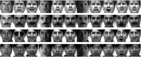
The YALE public image dataset was presented as a matrix and used to evaluate the KSTM performance through experiments. The dataset contains 165 100´100 face images of 15 people, 11 per person. Several typical images of YALE dataset are provided in Figure 1. It can be seen that the face images are grayscale images with 256 grayscale levels per pixel, all of which are directly stored as 2nd order tensors.
The images were not cropped or resized to avoid reducing the number of features in the original data, and all the features in the YALE dataset were scaled to the interval [0, 1], for the experiments aim to test the effectiveness of the KSTM in classifying the data expressed as 2nd order tensor for high-dimensional problems with a small sample size.
To evaluate the performance of tensor-based classifiers, two kinds of kernels were selected, namely the Gaussian-based kernel matrix and the polynomial-based kernel matrix. Taking the ij-th element for example, the Gaussian-based kernel matrix and the polynomial-based kernel matrix can be respectively defined as:
$\varphi\left(z_{i p_{1}}\right) \varphi\left(z_{j p_{1}}\right)^{T}=e^{-\left\|z_{i p_{1}}-z_{i p_{2}}\right\|^{2} / 2 \sigma^{2}}$ (25)
$\varphi\left(z_{i p_{1}}\right) \varphi\left(z_{j p_{1}}\right)^{T}=\left(z_{i p_{1}}^{T} z_{i p_{2}}+1\right)^{d}$ (26)
For clarity, the KSTMs with Gaussian-based and polynomial-based kernel matrices are denoted as gKSTM and pKSTM, respectively.
In addition, the two KSTMs were compared to the standard SVMs with Gaussian kernel function $k(x, y)=e^{-\|x-y\|^{2} / 2 \sigma^{2}}$ and polynomial kernel function $k(x, y)=\left(x^{T} y+1\right)^{d}$. The two types of KVSMs are denoted as gKSVM and pKSVM, respectively.
There are three tuning parameters: n , s and d. The possible choices for these parameters are v ={2-2, 2-1, 20, 21, 22, 23, 24, 25, 26, 27, 28, 29, 210}, s ={20, 21, 22, 23, 24, 25, 26, 27, 28, 29, 210} and d ={1, 2, 3, 4, 5, 6, 7, 8}.
All the four algorithms were implemented in MATLAB 7.0 on Windows 8.1 running on a personal computer (Intel Core i3 2.4 GHz; 8GB RAM).
Figure 1. Typical images of YALE dataset
4.2 Classification performance
The gKSTM, gKSVM, pKSTM and pKSVM were evaluated on YALE dataset. Since both the STM and the SVM are binary classification machine learning models, two types of training samples, positive and negative, were selected randomly for each experiment.
Ten random training samples are listed in Table 1. For example, (7, 13) means the 7th and 13th face images are used for the current set of experiments, in which the former is a positive sample and the latter, a negative sample.
In addition, the number of samples in the training set was strictly controlled to provide a small sample size. Here, the 4th, 6th, 8th, 10th and 12th face images are taken as training images. For the lack of space, only the classification results with 4 training samples are given in Table 1. The classification performance with training sets in other sizes will be discussed at the end of this section. In order to ensure the reliability of the results, the training set was divided randomly 10 times, and the final results are the average of 10 experiments for statistical significance.
Table 1 shows the mean classification accuracy of the STM and SVM algorithms on different training sets containing 4 samples, and the highest value is marked in bold. Obviously, the STM achieved better classification accuracy than the SVM in eight out of the ten groups of experiments, and realized poorer accuracy than the latter in the remaining two groups of experiments. Overall, the STM outperforms the SVM in the classification of a small number of sample images. In addition, the gSTM boasted the highest classification accuracy in six out of the eight groups of data, on which the STM outperformed the SVM.
Table 1. Mean accuracy on 10 random target classes in YALE dataset
|
Training Set |
Algorithm |
Accuracy |
Algorithm |
Accuracy |
Training Set |
Algorithm |
Accuracy |
Algorithm |
Accuracy |
|
(7,13) |
gSTM |
0.9778 |
gSVM |
0.6833 |
(6,7) |
gSTM |
0.9556 |
gSVM |
0.7778 |
|
pSTM |
0.9167 |
pSVM |
0.9167 |
pSTM |
0.9667 |
pSVM |
0.8722 |
||
|
lSTM |
0.9167 |
lSVM |
0.9611 |
lSTM |
0.9778 |
lSVM |
0.9167 |
||
|
(1,12) |
gSTM |
0.9389 |
gSVM |
0.7111 |
(1,4) |
gSTM |
0.9444 |
gSVM |
0.7167 |
|
pSTM |
0.8667 |
pSVM |
0.8944 |
pSTM |
0.9000 |
pSVM |
0.9056 |
||
|
lSTM |
0.8778 |
lSVM |
0.8944 |
lSTM |
0.9000 |
lSVM |
0.9056 |
||
|
(4,11) |
gSTM |
1.0000 |
gSVM |
0.7833 |
(5,6) |
gSTM |
0.8889 |
gSVM |
0.7444 |
|
pSTM |
0.9944 |
pSVM |
0.9944 |
pSTM |
0.9056 |
pSVM |
0.8722 |
||
|
lSTM |
0.9944 |
lSVM |
0.9944 |
lSTM |
0.8944 |
lSVM |
0.8722 |
||
|
(2,6) |
gSTM |
0.9000 |
gSVM |
0.7111 |
(3,15) |
gSTM |
0.8500 |
gSVM |
0.6722 |
|
pSTM |
0.8833 |
pSVM |
0.7944 |
pSTM |
0.8944 |
pSVM |
0.9056 |
||
|
lSTM |
0.8833 |
lSVM |
0.9000 |
lSTM |
0.8944 |
lSVM |
0.9056 |
||
|
(1,14) |
gSTM |
0.9333 |
gSVM |
0.7389 |
(6,12) |
gSTM |
0.7778 |
gSVM |
0.6778 |
|
pSTM |
0.8889 |
pSVM |
0.9056 |
pSTM |
0.8389 |
pSVM |
0.8833 |
||
|
lSTM |
0.8833 |
lSVM |
0.9056 |
lSTM |
0.8611 |
lSVM |
0.9167 |
Figure 2. Target class (7,13), Teat accuracy
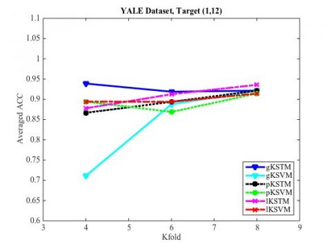
Figure 3. Target class (1,12), Teat accuracy
Figure 4. Target class (4,11), Teat accuracy
Figure 5. Target class (2,6), Teat accuracy
Figure 6. Target class (1,14), Teat accuracy
Figure 7. Target class (6,7), Teat accuracy
Figure 8. Target class (1,4), Teat accuracy
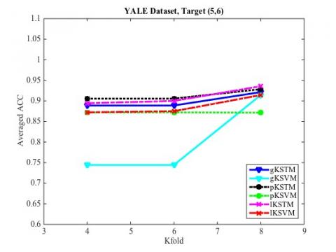
Figure 9. Target class (5,6), Teat accuracy
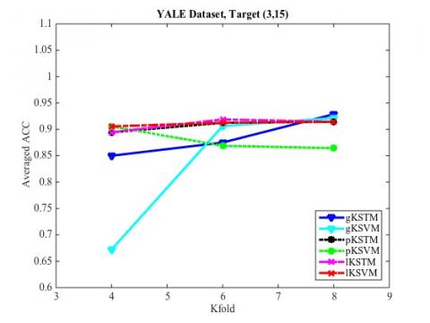
Figure 10. Target class (3,15), Teat accuracy
Figure 11. Target class (6,12), Teat accuracy
Figures 2-11 are the line charts of the relationship between the classification accuracy of the STM and SVM and the number of training samples obtained in the ten groups of experiments. It can be seen that, when the size of training samples was small, the STM had a much higher classification accuracy than the SVM; with the growing number of samples, the SVM exhibited roughly the same classification accuracy as the STM. Hence, the KSTM algorithm, which is based on tensor representation, is particularly suitable for solving high-dimensional problems with a small sample size.
This paper proposes a kernel-based support tensor machine (KSTM) based on tensor representation, and applies it to classify real-world images. To verify its performance, the KSTM was tested through classification experiments on the YALE face image datasets. The greatest advantage of our algorithm is the ability to maintain the integrity of tensor data, especially for high-dimensional problems with a small sample size. The KSTM also has better classification accuracy than linear algorithms.
Of course, there are some limitations with our algorithm. Despite having fewer decision variables than the vector classifier, the tensor classifier adopts the alternating projection algorithm in its STL framework, i.e. its training time depends on the iteration times of the alternating projection algorithm, which is often much higher than the vector model. Hence, the future research will try to optimize the KSTM algorithm and improve its training efficiency. Furthermore, further research will be carried out on the high-order KSTM.
The work is supported by The Research and Practice on The Through-Type Training Mode of High-End Technologies and Technical Skills Personnel of Beijing (Beijing Municipal Education Commission, Beijing, China, Grant No. 2018-54), The Famous Teacher of Beijing and The Academic Research Project of Beijing Union University (ZK50201902).
[1] Tao, D., Li, X., Wu, X., Hu, W., Maybank, S.J. (2007). Supervised tensor learning, knowledge and information systems. Knowledge and Information Systems, 13(1): 1-42.
[2] Mistani, P., Pakravan, S., Gibou, F. (2019). Towards a tensor network representation of complex systems. In Sustainable Interdependent Networks II, 69-85. https://doi.org/10.1007/978-3-319-98923-5_4
[3] Gupta, S., Thirukovalluru, R., Sinha, M., Mannarswamy, S. (2018). CIMTDetect: A community infused matrix-tensor coupled factorization based method for fake news detection. In 2018 IEEE/ACM International Conference on Advances in Social Networks Analysis and Mining (ASONAM), Barcelona, Spain, pp. 278-281. https://doi.org/10.1109/ASONAM.2018.8508408
[4] Lanini, M., Ram, A. (2019). The Steinberg-Lusztig tensor product theorem, Casselman-Shalika, and LLT polynomials. Representation Theory of the American Mathematical Society, 23(5): 188-204. https://doi.org/10.1090/ert/524
[5] Benaroya, E.L., Obin, N., Liuni, M., Roebel, A., Raumel, W., Argentieri, S. (2018). Binaural localization of multiple sound sources by non-negative tensor factorization. IEEE/ACM Transactions on Audio, Speech, and Language Processing, 26(6): 1072-1082. https://doi.org/10.1109/TASLP.2018.2806745
[6] Kotsia, I., Guo, W., Patras, I. (2012). Higher rank support tensor machines for visual recognition. Pattern Recognition, 45(12): 4192-4203. https://doi.org/10.1016/j.patcog.2012.04.033
[7] Zhang, X., Gao, X., Wang, Y. (2009). Twin support tensor machines for MCs detection. Journal of Electronics (China), 26(3): 318-325. https://doi.org/10.1007/s11767-007-0211-0
[8] Chen, Y., Wang, K., Zhong, P. (2016). One-class support tensor machine. Knowledge-Based Systems, 96: 14-28. https://doi.org/10.1016/j.knosys.2016.01.007
[9] Chen, Y., Lu, L., Zhong, P. (2017). One-class support higher order tensor machine classifier. Applied Intelligence, 47(4): 1022-1030. https://doi.org/10.1007/s10489-017-0945-9
[10] Biswas, S.K., Milanfar, P. (2017). Linear support tensor machine with LSK channels: Pedestrian detection in thermal infrared images. IEEE Transactions on Image Processing, 26(9): 4229-4242. https://doi.org/10.1109/TIP.2017.2705426
[11] Cao, B., He, L., Wei, X., Xing, M., Yu, P.S., Klumpp, H., Leow, A.D. (2017). t-BNE: Tensor-based brain network embedding. In Proceedings of the 2017 SIAM International Conference on Data Mining, Society for Industrial and Applied Mathematics, pp. 189-197. https://doi.org/10.1137/1.9781611974973.22
[12] Cichocki, A., Mandic, D., De Lathauwer, L., Zhou, G., Zhao, Q., Caiafa, C., Phan, H.A. (2015). Tensor decompositions for signal processing applications: From two-way to multiway component analysis. IEEE Signal Processing Magazine, 32(2): 145-163. https://doi.org/10.1109/MSP.2013.2297439
[13] Guo, T., Han, L., He, L., Yang, X. (2014). A GA-based feature selection and parameter optimization for linear support higher-order tensor machine. Neurocomputing, 144: 408-416. https://doi.org/10.1016/j.neucom.2014.05.018
[14] Lu, C.T., He, L., Shao, W., Cao, B., Yu, P.S. (2017). Multilinear factorization machines for multi-task multi-view learning. In Proceedings of the Tenth ACM International Conference on Web Search and Data Mining, pp. 701-709. https://doi.org/10.1145/3018661.3018716
[15] Krawczyk, B., Galar, M., Woźniak, M., Bustince, H., Herrera, F. (2018). Dynamic ensemble selection for multi-class classification with one-class classifiers. Pattern Recognition, 83: 34-51. https://doi.org/10.1016/j.patcog.2018.05.015
[16] Cai, D., He, X.F., Han, J.W. (2006). Learning with tensor representation. Illinois Digital Environment for Access to Learning and Scholarship, UIUCDCS-R-2006-2716. http://hdl.handle.net/2142/11195
[17] Signoretto, M., De Lathauwer, L., Suykens, J.A. (2011). A kernel-based framework to tensorial data analysis. Neural Networks, 24(8): 861-874. https://doi.org/10.1016/j.neunet.2011.05.011
[18] He, L., Kong, X., Yu, P.S., Yang, X., Ragin, A.B., Hao, Z. (2014). Dusk: A dual structure-preserving kernel for supervised tensor learning with applications to neuroimages. In Proceedings of the 2014 SIAM International Conference on Data Mining, Society for Industrial and Applied Mathematics, pp. 127-135. https://doi.org/10.1137/1.9781611973440.15
[19] Pilarczyk, R., Chang, X., Skarbek, W. (2019). Human face expressions from images-2D face geometry and 3D face local motion versus deep neural features. arXiv preprint arXiv:1901.11179.
[20] Gao, C., Wu, X.J. (2012). Kernel support tensor regression. Procedia Engineering, 29: 3986-3990. https://doi.org/10.1016/j.proeng.2012.01.606
[21] Daniušis, P., Vaitkus, P. (2008). Kernel regression on matrix patterns. Lithuanian Mathematical Journal. Spec. Edition, 49: 191-195.
[22] Park, S.W. (2011). Multifactor analysis for FMRI brain image classification by subject and motor task. Electrical and Computer Engineering Technical Report.
[23] Chen, Z.Y., Fan, Z.P., Sun, M. (2016). A multi-kernel support tensor machine for classification with multitype multiway data and an application to cross-selling recommendations. European Journal of Operational Research, 255(1): 110-120. https://doi.org/10.1016/j.ejor.2016.05.020
[24] Alharbi, S.S., Sazak, Ç., Nelson, C.J., Obara, B. (2018). Curvilinear structure enhancement by multiscale top-hat tensor in 2D/3D images. In 2018 IEEE International Conference on Bioinformatics and Biomedicine (BIBM), Madrid, Spain, Spain, pp. 814-822. https://doi.org/10.1109/BIBM.2018.8621329
[25] Diaz, P., Rey, S.J. (2018). Invariant operators, orthogonal bases and correlators in general tensor models. Nuclear Physics B, 932: 254-277. https://doi.org/10.1016/j.nuclphysb.2018.05.013
[26] Bonzom, V., Nador, V., Tanasa, A. (2019). Diagrammatics of the quartic O (N) 3-invariant Sachdev-Ye-Kitaev-like tensor model. Journal of Mathematical Physics, 60(7): 072302. https://doi.org/10.1063/1.5095248
[27] David, A., Lerner, B. (2005). Support vector machine-based image classification for genetic syndrome diagnosis. Pattern Recognition Letters, 26(8): 1029-1038. https://doi.org/10.1016/j.patrec.2004.09.048
[28] Patel, A.K., Chatterjee, S., Gorai, A.K. (2019). Effect on the Performance of a support vector machine based machine vision system with dry and wet ore sample images in classification and grade prediction. Pattern Recognition and Image Analysis, 29(2): 309-324. https://doi.org/10.1134/S1054661819010097