Qiao Huang | Limin Cui*
OPEN ACCESS
Face recognition is a promising technology with a great application potential and broad prospects for development. Compared with other identification technologies, face recognition can achieve rapid and easy sampling, without affecting the behavior of the sampled. These advantages have induced a surging demand and interests in this technology, making it a research hotspot in artificial intelligence. This paper extracts the features from the target face image by Principal Component Analysis (PCA), reducing the dimension of the image. Taking the feature coordinates of the face image for classification, it is possible to eliminate the excess computing load induced by high dimensionality. After that, the backpropagation (BP) neural network was improved by the scaled conjugate gradient (SCG) algorithm. The improvement aims to control the model error caused by the defects of the original BP neural network, including inefficient learning, slow convergence and proneness to local minimum. The improved BP neural network was then adopted to classify the feature coordinates of the face image. Finally, the proposed face recognition algorithm was implemented on Matlab and trained with the improved BP neural network. The experimental results show that the proposed algorithm achieved good recognition performance.
face recognition, backpropagation (BP) neural network, principal component analysis (PCA), image feature extraction, scaled conjugate gradient (SCG) algorithm
The rapid development of society and the popularization of computer and network increase the demand for convenient, reliable and stable identity recognition. At present, there are many kinds of identity recognition methods. Among them, the recognition method based on biological morphological features is a research hotspot. The biological characteristics of each person are attributes possessed by himself or herself, and these biological characteristics are stable in each person but greatly different for different individuals, which are needed for the identification. Biometric technologies include fingerprint recognition, voice recognition, face recognition, iris recognition, gait recognition, and so on [1]. Compared with many other identification technologies, however, the face recognition technology has high security, wide application range and strong practicability and has been widely used in login verification, attendance check, community security, video monitoring, judicial enforcement, and other popular and important areas. Therefore, the face image recognition technology with high computation speed, convenient sampling and high recognition accuracy has wide research value and application prospect.
After decades of rapid development, there have been many theoretical research results obtained in the field of computer face image recognition. Francis Galton published two articles on the use of face images for identification on the Nature in 1888 and 1910, respectively [2]. In the studies on face recognition, he tried to quantify the side face information of a face image with a set of numbers and then carry out the face image recognition with the obtained side face information as a feature. Francis Galton can be said to be a pioneer of face recognition. However, due to the slow development of the fields related to face recognition, especially the computer field, Francis Galton's research has not been paid much attention to [3].
One of the difficulties faced by face recognition is that face images of faces vary greatly with many external conditions. Although human beings can easily avoid these external interferences to recognize face images, it is very difficult to implement this function using a computer. The extensive research of face recognition originated in the 1960s, and Bledsoe and Chan published a technical report on automatic face recognition at Panoramic Research Inc. in 1965 [4], which is a well-recognized opening in the academic world of face recognition research. However, this is a semi-automatic method that relies on a priori knowledge of the operator, needs a professional to manually extract feature point, and then performs computer recognition. There is a rapid development of research on face image recognition since 1990 [5].
In 1991, Turk, Pentland and other scholars at the Massachusetts Institute of Technology introduced the Principal Component Analysis (PCA) method to face recognition and proposed the famous Eigenface method [6], which has greatly promoted the progress of face recognition as a classical algorithm of face recognition. PCA is a method of KL transformation (Karhunen and Loeve Transformation). It is simple in principle, easy in programming, fast in speed, good in identification and efficient in solving practical problems. However, the PCA method depends on the gray correlation of the image itself, so the recognition rate is poor when the background, light and position are different. In the face recognition field, this process can realize the real automatic recognition of the face image, which is a big leap of face image recognition.
The BP neural network algorithm proposed by Rumelhart et al. in 1986 has become one of the most widely used neural network models, because BP neural network can extend the knowledge learned from some samples to all the samples; when the number of samples is sufficient, it has the functions of association, self-adaptation or self-learning; it can automatically summarize the law in the updating of the weights; the local error will not be subversive to all the research samples, so it can solve the problem of insufficient information. The essence of face recognition is a classification issue, in which BP neural network is widely used as a classifier, and this study uses the BP neural network as a classifier for face images, which is of great theoretical value and practical significance in face recognition [7-11]. BP neural network, however, has a slow learning rate; it takes too much time to train the weights of neural networks; it is easy to be affected by local minimum, so that the network error is too large, which leads to the low recognition rate. Face image is usually a high-dimensional vector when data is input, so face recognition of BP neural network often has too much computing load and slow error convergence speed, and its recognition success rate does not meet the requirements.
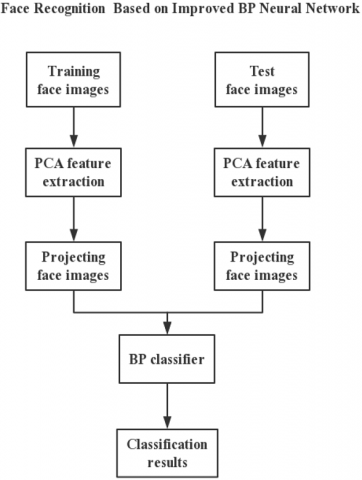
This paper firstly uses PCA to reduce the dimension of the image, extracts the average face and eigenface image vectors, and then obtains the projection coordinates of each image with reduced dimension on the eigenface face. BP neural network is used to realize the classification of the projection coordinates, with good classification results obtained. SCG algorithm is used to optimize BP neural network, and applied to face recognition of BP neural network, so as to greatly improve the correctness and convergence efficiency of BP neural network for face recognition. Finally, for different parameters, experiments are carried out with different number of samples and different face databases. The flow chart of the whole system is shown in Figure 1.
Figure 1. Flow chart of the whole system
2.1 BP algorithm
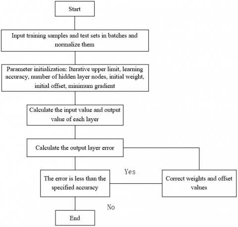
The neural network can obtain a set of output vectors from the input vectors, but since the initial weights and the offset values of the neural network are given randomly, the designed neural network is only making some random judgments and cannot operate in the way we expect. Therefore, we must "train" the neural network to achieve the goal of "learning." As a common method in machine learning, neural network has many ways of learning. The BP (Back Propagation) algorithm is studied in this paper. The flow chart of BP neural network algorithm is shown in Figure 2.
Figure 2. Flow chart of BP neural network algorithm
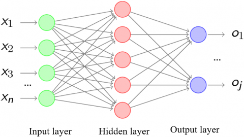
In the BP neural network, several layers (one or more layers) of neurons are added between the input layer and the output layer, these neuron are called hidden units, which have no direct connection with the outside world, but the change of their states can influence the relationship between the input and the output, and each layer may have several nodes. A three-layer BP neural network is shown in Figure 3.
Figure 3. Topology of BP neural network
The basic implementation flow of the BP neural network is as follows: when a sample is input, first obtain the eigenvector of the sample, and then the input value of the perceptron according to the weight vector; calculate the output of each perceptron with the sigmoid function; use this output as the input to the next layer perceptron, and so on, up to the output layer. In this process, the input weight vector can be continuously adjusted by minimizing the loss function, and then the weight is adjusted layer by layer from back to front, which is the idea of the back propagation algorithm.
The back propagation algorithm for a feedforward network with two layers of sigmoid function is defined as follows:
(1) Random initialization of the ownership value in the network.
(2) For each training sample, the output of each unit in the output layer is calculated sequentially from the front to the back according to the input of the examples. The error term for each unit of each layer is then computed back from the output layer. For each unit k of the output layer, its error term is calculated: δk=ok (1-ok)(tk-ok).
For each hidden unit h in the network, its error term is calculated: ${{\delta }_{h}}={{o}_{h}}(1-{{o}_{h}})\sum\nolimits_{k\in outputs}{{{w}_{kh}}{{\delta }_{h}}}$, where outputs represents a set of output layer nodes, and wkh represents the corresponding weight.
(3) Update each weight: wji=wji+∆wji, where ∆wji is known as the weight update rule.
2.2 Improved BP neural network
In the process of using BP neural network to deal with practical problems, especially in complex problems where the dimension of input sample vector is too high, the convergence speed of the neural network model is slow. Because the updating weight falls into the local minimum, which leads to too large error and other problems that cannot be ignored. Therefore, the improved BP algorithm is often used to update the weight in the practical application.
This paper uses SCG algorithm to improve the BP neural network of face recognition. SCG algorithm originates from the improvement of conjugate gradient algorithm. The difference between SCG algorithm and conjugate gradient algorithm is that when searching step size is calculated with another method to accurately calculate the search step size instead of the linear search method of the conjugate gradient algorithm, and the SCG also guarantees the positive nature of the Hessian matrix [12].
The conjugate gradient algorithm and the SCG algorithm will be described in detail below.
2.2.1 Principle of conjugate gradient algorithm
The conjugate gradient algorithm uses the gradient vector to calculate the conjugate direction, so the convergence speed will be faster than the steepest descent algorithm [9]. There are many kinds of conjugate gradient algorithms. However, the iteration of all method begins with the search direction determined by the steepest descent algorithm, i.e., p0=-g0, where g0 represents the gradient direction and one-dimensional search is carried out firstly according to the linear search method: wk+1=wk+akpk, where ak represents the search step size, which can be calculated with $\min _ { a _ { k } \geq 0 } f \left( w _ { k } + a _ { k } p _ { k } \right)$.
Assume the negative direction of gradient of pk is -gk, the next search direction is the conjugate direction of the previous search, and the direction vector calculated by the conjugate gradient algorithm is as follows: pk=-gk+βkpk-1.
2.2.2 Principle of Scaled Conjugate Gradient (SCG) algorithm
In the conjugate gradient algorithm, the search step size ak is calculated with $\min _ { a _ { k } \geq 0 } f \left( w _ { k } + a _ { k } p _ { k } \right)$.
The formula: $a _ { k } = \frac { g _ { k } ^ { T } p _ { k } } { p _ { k } ^ { T } H _ { k } p _ { k } }$.
Assume $s _ { k } = E ^ { \prime \prime } \left( w _ { k } \right) p _ { k } , \delta _ { k } = p _ { k } ^ { T } s _ { k }$ and $u _ { k } = - g _ { k } ^ { T } p _ { k }$, then the above formula can be written as: $a_k=frac{u_k}{\delta_k}$.
In SCG, the formula of sk is as follows: $S _ { k } = \frac { E ^ { \prime } \left( w _ { k } + \sigma _ { k } p _ { k } \right) - E ^ { \prime } \left( w _ { k } \right) } { \sigma _ { k } } + \lambda _ { k } p _ { k }$, where λk is called scale factor. The positive definite of the Hessian Matrix can be ensured by adjusting the value of λk.
The adjusted value of λk is $\overline { \lambda } _ { k }$, the adjusted value of sk is $\overline { s } _ { k }$ and the formula of calculating $\overline { s } _ { k }$ is: $\overline { s } _ { k } = s _ { k } + \left( \overline { \lambda } _ { k } - \lambda _ { k } \right) p _ { k }$.
In the process of iteration, if δk≤0, the Hessian Matrix is not positive definite and can be adjusted by setting λk to make δk>0, and the adjusted value of δk as $\overline { \delta } _ { k }$, then the formula: $\overline { \delta } _ { k } = p _ { k } ^ { T } \overline { s } _ { k } = p _ { k } ^ { T } \left( s _ { k } + \left( \overline { \lambda } _ { k } - \lambda _ { k } \right) p _ { k } \right) = \delta _ { k } + \left( \overline { \lambda } _ { k } - \lambda _ { k } \right) \left| p _ { k } \right| ^ { 2 } > 0$.
Calculate: $\overline { \lambda } _ { k } > \lambda _ { k } - \frac { \delta _ { k } } { \left| p _ { k } \right| ^ { 2 } }$.
Therefore, the scale factor λk can adjust the length of the step in the calculation and ensure the positive definiteness of the Hessian Matrix, and in the SCG algorithm, the parameters λ and σ need to be initialized. In the algorithm, λ will be automatically adjusted, so the value is random, less than or equal to 10-6. Once σ is determined in the initialization, it remains unchanged, and thus σ affects the performance of the algorithm to a certain extent, that’s, the smaller theoretically it is, the higher the accuracy of the algorithm is. It has been shown that σ is small enough in experiments (σ<10-4), but has little effect on the algorithm, which implies the strong stability of SCG algorithm [14].
3.1 Feature extraction of face images
In recognizing face images, the first problem is the complexity of the images. If the pixel of face images is the gray scale 92x122, the extraction method input to the computer is first column and then row, that’s, from top to bottom. The pixel values of the images are sequentially extracted from left to right, resulting in a vector of 10304 dimensions. If this vector is directly used as the input of BP neural network classifier, too high dimension of input value will lead to the problems of slow calculation and too large error due to too many parameters. Because of the similarity structure of the face image, there must be a lot of redundancy in the description of the vector of 10304 dimension, that’s, the values in different dimensions of the vector of 10304 dimension may be the expression of the same information, and therefore it’s meaningful to extract the key features of each image for identification
In order to improve the recognition rate and accuracy of BP neural network, PCA is used to reduce the dimension of low-frequency components of face images obtained after discrete wavelet transform and extract principal component features. With the PCA method, a relatively small number of eigenvectors with high information content can be extracted from the original face image data, and this eigenvector vector is also referred to as eigenface. The projection of each face image vector on the eigenface is calculated. Finally, the feature of each face image is described by the projection vector coordinates of each image. This process realizes the feature extraction of the face image. In this process, the original face image can be approximately expressed as a linear combination of the coordinate of each face image and the eigenface, and the BP neural network classifier pair will be trained by using the eigenvector of the face image, so as to realize the recognition of the eigenvector of the face image of the test sample by the BP neural network classifier.
With PCA algorithm, it’s possible to replace the original high-dimensional face image vector with the low-dimensional face eigenvector, which still can represent most of the information of the original image. The original m-dimension vector can be projected to the u-dimension based on the selected eigenface, while the linear combination of the u-dimension coordinate vector and the eigenface can describe the original face image while ensuring u- and m-dimension vector. Therefore, the u-dimension coordinate vector shows the comprehensive effect of the original face image, effectively retains the features of the original face images, and greatly reduces the repetition rate and dimension of the data.
Assuming that the i-th face image vector is Xi, if there are n face images, the dimension of each face image is m, so the face images can be represented as X1,X2,…,Xn and set a sample matrix as X=(X1,X2,…,Xn), and the algorithm flow of extracting features using principal components of PCA is as follows
(1) Calculate the covariance matrix S of the sample X, first centralize the data, that’s, obtaining the average value of each column $\overline { X } = \frac { 1 } { n } \sum _ { i = 1 } ^ { n } X _ { i }$, in which the average of all face images can be described as $\overline{X}$, namely, the average face.
(2) Centralize each face image: $X _ { i } - \overline { X } , i = 1,2 , \cdots n$.
Record the centralized sample as: $A = \left( X _ { 1 } - \overline { X } , X _ { 2 } - \overline { X } , \cdots X _ { n } - \overline { X } \right)$.
(3) Through the conclusion of the singular value decomposition of the formula, in order to obtain the eigenvector ui, first calculate C as follows: C=ATA, where the matrix C is a nxn matrix.
(4) Calculate the eigenvalue λ1,λ2,…,λm of the covariance matrix S and the corresponding eigenvectors: v1,v2,…,vm.
Calculate the cumulative contribution rate p according to the formula $p = \frac { \sum _ { i = 1 } ^ { u } \lambda _ { i } } { \sum _ { i = 1 } ^ { m } \lambda _ { i } }$, sort λ1,λ2,…,λu from the large to the small, and select the u feature values with 90% of the cumulative contribution rate from the large to the small.
(5) Select the first u eigenvalues from large to small to get the corresponding eigenvector v1,v2,…,vu, $u _ { i } = \frac { 1 } { \sqrt { \lambda _ { i } } } A v _ { i }$, i=1,2,…u, and u eigenvectors are used to form the matrix Z.
The form of Z is:
$Z = \left[ \begin{array} { c } { u _ { 1 } } \\ { u _ { 2 } } \\ { \vdots } \\ { u _ { u } } \end{array} \right] ^ { 7 }$.
(6) Calculate the projection of each sample on the matrix Z, with the formula as follows: W=ATZ.
The obtained row vector of W is the eigenvector of each face image, and this process completes the feature extraction of the face image. In the W matrix, the number of rows corresponds to the image samples, and the number of columns corresponds to the dimension of the extracted features of the images, reducing the m-dimension face image vector to the u-dimension face image eigenvector.
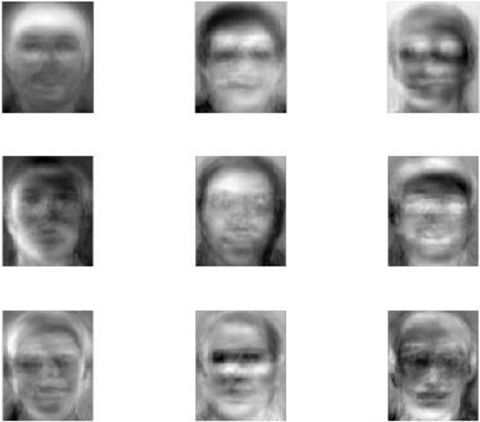
PCA feature extraction is to use PCA algorithm to make principal component analysis on the matrix consisting of gray values of face images, so as to realize face feature extraction. Eigenface images are as shown in Figure 4.
Figure 4. Eigenface images
3.2 Design of BP neural network for face image recognition
Because the face recognition by BP neural network realizes the mapping from the input face eigenvector to the output classification vector, only the training set of the face image library is needed in practice to train the neural network according to the BP algorithm, so that the error of the neural network can be gradually reduced and the ability to map correctly from input to output can be achieved.
BP neural network takes the form of supervised learning, so the input data format is: (input vector and label).
The input vector is the face image vector $\vec{x}$ after the feature extraction, and the vector $\vec{x}$ is reduced to M dimension through the feature extraction process in this paper. The following mainly divides into two stages to realize the face image recognition of the BP neural network:
(1) Perform an initialization operation on the defined neural network
The ownership weight matrix W(1),W(2),..,W(n) of neurons in each layer of the neural network is randomly initialized, wherein each weight is taken to a random value near 0. Define the activation function f1,f2,…,fn of neurons in each layer of the neural network, whereby a neural network is generated. However, because of the randomness of the assignment, the output result of this network is also making random judgment. Only by selecting the training set of face image eigenvectors to train this network, can the neural network make the correct judgment
(2) The forward propagation process of face image eigenvector in the neural network
a) Take a data from the sample set and set the p-th data taken out, with the form as (${{\vec{x}}^{p}}$,${{\vec{t}}^{p}}$), and face image eigenvector ${{\vec{x}}^{p}}$ is input into the neural network as the initial value of the input layer. The forward propagation process of the neural network can be realized with $\vec{a}=f({{\vec{x}}^{p}}\cdot W)$, where $\vec{a}$ is the output of the neuron in the layer of the neural network, f is activation function, and W is the weight matrix among layers of the neural network.
b) The formula $\vec{a}=f({{\vec{x}}^{p}}\cdot W)$ is used multiple times between layers until the output value ${{\vec{o}}^{p}}$ of the neural network is obtained. Assuming that there are n-layers of the neural network in total, the calculation process formula of the neural network is as follows: $\vec { o } ^ { p } = f _ { n } \left( \cdots \left( f _ { 2 } \left( f _ { 1 } \left( \vec { x } ^ { p } W ^ { ( 1 ) } \right) W ^ { ( 2 ) } \right) \cdots \right) W ^ { ( n ) } \right)$, where f1,f2,…,fn is an activation function corresponding to each layer and W(1),W(2),..,W(n) is the weight matrix corresponding to each layer. The resulting output vector ${{\vec{o}}^{p}}$ is the result of the forward propagation process.
c) Calculate the minimum mean square error of each sample, calculate the minimum mean square error of ${{\vec{o}}^{p}}$ with the label of all face image samples, and take the vector $\vec{t}$ with the smallest error as the result of this recognition. The coordinate with the ${\vec{t}}$ position of 1 is the mark of each image from the definition of ${\vec{t}}$, with the result of this face recognition obtained.
(3) Back-propagation algorithm for face image recognition
The error function of the neural network is defined by using the errors of all the samples in the training set, and the calculation formula of the total error E is obtained as below: $E = \sum _ { p = 1 } ^ { P } E _ { p } = \frac { 1 } { 2 } \sum _ { p = 1 } ^ { P } \sum _ { k = 1 } ^ { L } \left( T _ { k } ^ { p } - o _ { k } ^ { p } \right) ^ { 2 }$, where P is the number of eigenvectors of the face images included in the training set, $T^P_K$ is the desired output of the k-th position of the eigenvector sample p of each face image, and $o^P_K$ is the actual output of the k-th position of the eigenvector sample p of each face image.
a) Train the weights of the output layer
After the total error E of the neural network is calculated, the partial derivative $\frac { \partial E } { \partial w _ { k i } }$ of the error E with respect to each weight of the output layer can be calculated:
$\frac { \partial E } { \partial w _ { k i } } = - \sum _ { p = 1 } ^ { P } \sum _ { l = 1 } ^ { L } \left( T _ { l } ^ { p } - o _ { l } ^ { p } \right) \psi ^ { \prime } \left( n e t _ { k } \right) x _ { k i }$.
This formula can be used to calculate the gradient vector of the output layer weight.
b) Train the weights of the hidden layer
In a similar way to train the weights of the output layer, that’s, calculate the partial derivative $\frac { \partial E } { \partial w _ { k i } }$ of the error E with respect to each weight of the hidden layer, then $\frac { \partial E } { \partial w _ { i j } } = \sum _ { p = 1 } ^ { P } \sum _ { l = 1 } ^ { L } \left( T _ { l } ^ { p } - o _ { l } ^ { p } \right) \psi ^ { \prime } \left( n e t _ { k } \right) w _ { k i } \phi ^ { \prime } \left( n e t _ { i } \right) x _ { j }$.
This formula can be used to calculate the gradient vector of the hidden layer weight.
c) Calculate the size of each weight adjustment
Set the learning rate of the gradient descent method, and set the correction amount of the output layer weight as ∆wki and the correction amount of the hidden layer weight as ∆wij, wherein the correction amount of the output layer weight as:
$\Delta w _ { k i } = - \eta \frac { \partial E } { \partial w _ { k i } } = \eta \sum _ { p = 1 } ^ { P } \sum _ { l = 1 } ^ { L } \left( T _ { l } ^ { p } - o _ { l } ^ { p } \right) \psi ^ { \prime } \left( n e t _ { k } \right) x _ { k i }$.
And the correction amount of the hidden layer weight as:
$\Delta w _ { i j } = - \eta \frac { \partial E } { \partial w _ { i j } } = \eta \sum _ { p = 1 } ^ { P } \sum _ { l = 1 } ^ { L } \left( T _ { l } ^ { p } - o _ { l } ^ { p } \right) \psi ^ { \prime } \left( \text {net} _ { k } \right) w _ { k i } \phi ^ { \prime } \left( \text {net} _ { i } \right) x _ { j }$.
d) Adjust weight by gradient descent method
After defining the error function E, in order to reduce the error function, a gradient descent algorithm is used for optimization, with the formula as follows:
w(n+1)=w(n)+ ∆w(n).
w(n+1) represents the n+1-th weight; w(n) represents the n-th weight. This formula modifies the weight in the reverse direction of the gradient and is the direction in which the error function E is reduced most quickly.
e) Conditions for the termination of the training process
Using a sample set of eigenvectors of face images, the general training process termination condition is that the total error E of the model satisfies: E≤εP, where εP is an error limit defined as a set of samples, and the training process is terminated when the model error is less than this value. However, in the actual running process of the program, because the error cannot converge to the specified precision, the program will go on indefinitely, and the threshold value of the gradient is often set as ε, when all $\frac { \partial E } { \partial w }$ satisfy, $\frac { \partial E } { \partial w } \leq \varepsilon$. then the iteration is then terminated. In the course of program running, it is also possible to always meet situation such as failure to meet E≤εP or $\frac { \partial E } { \partial w } \leq \varepsilon$. In order to avoid this situation, it is also necessary to set the upper limit N of the number of iteration times, update the formula of the weighted value: w(n+1)=w(n)+ ∆w(n).
The iteration is terminated when meeting n>N. When any one of the three training conditions is satisfied, the training process ends, the weight data of the network at this time is recorded, and a neural network model calculated by the BP algorithm is obtained at this time.
4.1 Some notes
In the case of using the BP neural network as the classifier, the selection of the input lay nodes should be consistent with the dimension of the eigenvector of the original face image. It is assumed that the face eigenvector of 57 dimensions has been extracted in the process of feature extraction of the face image, so the number of input layer nodes of BP neural network should be 57.
The number of output layer nodes of BP neural network should be consistent with the number of classification. If there are 40 images in the face database, since the number of output layer nodes of BP neural network should be consistent with the number of classification, the number of output layer nodes of BP neural network in this experiment is 40.
For the design of the hidden layer, there is the following empirical formula [15]:
$n _ { 1 } = \sqrt { n + m } + \alpha , \cdot n _ { 1 } = \log _ { 2 } n$, where n represents the number of neurons in the input layer, m represents the number of neurons in the output layer, and α usually takes the constant between 1 and 10. However, the empirical formula only provide some reference, and the specific settings are tested according to the problem solved. After determining the input layer, output layer, activation function, and learning mode of the BP neural network, the recognition rate and iteration times of the training samples and the test samples are calculated by changing the number of neurons in the hidden layer, after the calculation results converge, to first select the number of neurons in the hidden layer with high recognition rate, easy convergence of the network and less iteration times. The test results under different neurons are shown in Table 1.
Therefore, considering the above factors comprehensively, when the number of neurons in the hidden layer is selected to be 50, the recognition rate is high, and the convergence speed is relatively fast.
After the training data set of the neural network and the connection structure of the neural network itself are determined, the output value and the total error value of the neural network are completely determined by the activation function, and for each neuron, its activation state is determined by the size of the output value calculated by the activation function. In the BP neural network design of face recognition, both the hidden layer and the output layer use the sigmoid function as the activation function, which is easier to train than the linear function, that’s, reducing the model error more quickly.
Table 1. Test table of number of hidden layer neurons
|
Number of hidden layer nodes |
Training set recognition rate |
Test set recognition rate |
Iteration times |
|
20 |
100 % |
86 % |
1707 |
|
30 |
100 % |
90 % |
1328 |
|
40 |
100 % |
92.5 % |
1757 |
|
50 |
100 % |
94.5 % |
1425 |
|
60 |
100 % |
93.5 % |
1217 |
|
70 |
100 % |
93 % |
1474 |
|
80 |
100 % |
93.5 % |
1061 |
|
90 |
100 % |
94 % |
1759 |
|
100 |
100 % |
94 % |
1560 |
|
110 |
100 % |
93 % |
1067 |
|
120 |
100 % |
93.5 % |
1612 |
In the calculation process of the neural network, the output value of each neuron is expected to approach 0 with the calculation of the activation function Sigmoid and can be adjusted in the region where the function derivative is larger. When the initial weight herein is between [0,0.1], the offset value is set in between [0,0.2], which can effectively avoid the problem that the weight value and the offset value are too large to converge.
4.2 Experimental results
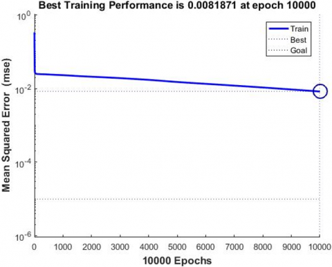
ORL (Olivetti Research Laboratory) face database is used in this experiment. The face database includes 40 people of different ages, genders and races. For each person, 10 images are extracted, with a total of 400 112 * 92 grayscale images. First, the first 5 images of each person are selected as training samples, and the last 5 images are taken as test samples to calculate the recognition result. In the face recognition experiment, the BP neural network of gradient descent algorithm is compared with the improved BP neural network of SCG algorithm adopted in this paper, and the BP neural network is trained and plotted by MATLAB. The mean square error maps of the neural network model for face recognition are shown in Figures 5 and 6.
Figure 5 is the mean square error descent curve of the gradient descent method, and Figure 6 is the improved mean square error descent training curve of the SCG algorithm. It can be seen that the model error of the gradient descent method is only about 10,000 iterations later is only about 10-2 while the SCG algorithm achieves 10-25 after 1595 iterations, so the SCG algorithm improves the BP neural network, speeds up the training speed and improves the accuracy of the BP neural network face recognition model.
In the ORL face database, from 10 face images of each person, 5 are randomly selected as training samples, the remaining 5 are used as test sets, weights and offset values are randomly assigned, 90% of the principal components are selected, the learning rate is 0.1, the model error is 10-15, the minimum gradient requirement is 10-15 and the upper limit of the number of iterations are 10,000. Due to the randomness of the experiment, 20 experiments are conducted in order to obtain more realistic performance test results of the algorithm. The experimental results are as shown in Table 2.
Figure 5. Model error curve of gradient descent method
Figure 6. Model error curve of SCG
It can be seen from the experimental results in Table 2 that the average recognition rate of the training set and the test set selected randomly is 95.18% and the average number of iterations is 1,696. The improved SCG algorithm has good recognition effect and convergence speed in ORL face database.
Then, the algorithm is verified by using Yale face database. From 11 face images of each person in Yale face database, 5 face images are randomly selected as training samples, and the remaining 6 face images are used as test sets, and weights and offset values are randomly assigned, selecting 90% of the principal component, learning rate of 0.1, model error of 10-25, minimum gradient requirement of 10-25, and the upper limit of the number of iterations of 10,000. Due to the randomness of this experiment, in order to obtain more realistic algorithm performance test results, 20 experiments were conducted, and the experimental results are as shown in Table 3.
Table 2. Experimental results of face recognition of ORL face database
|
Number of experiments |
Recognition rate of training samples |
Recognition rate of test samples |
Iteration times |
Number of extracted principal components |
|
1 |
100% |
94.5% |
2461 |
63 |
|
2 |
100% |
97% |
639 |
60 |
|
3 |
100% |
95% |
2916 |
61 |
|
4 |
100% |
94% |
624 |
64 |
|
5 |
100% |
94.5% |
1896 |
62 |
|
6 |
100% |
97% |
1461 |
60 |
|
7 |
100% |
95% |
1384 |
61 |
|
8 |
100% |
92.5% |
1865 |
62 |
|
9 |
99.5% |
95.5% |
1443 |
61 |
|
10 |
100% |
92% |
1517 |
62 |
|
11 |
100% |
95.5% |
2810 |
63 |
|
12 |
100% |
96.5% |
2453 |
59 |
|
13 |
100% |
95.5% |
482 |
62 |
|
14 |
100% |
96% |
3042 |
59 |
|
15 |
100% |
92.5% |
865 |
60 |
|
16 |
100% |
98% |
1540 |
61 |
|
17 |
100% |
97.5% |
1206 |
61 |
|
18 |
100% |
95% |
3567 |
59 |
|
19 |
100% |
96% |
808 |
61 |
|
20 |
100% |
94% |
934 |
59 |
|
Number of experiments |
Recognition rate of training samples |
Recognition rate of test samples |
Iteration times |
Number of extracted principal components |
|
1 |
100 % |
88 % |
1093 |
25 |
|
2 |
100 % |
96 % |
510 |
27 |
|
3 |
97.78 % |
96 % |
1554 |
24 |
|
4 |
100 % |
98.67 % |
473 |
23 |
|
5 |
100 % |
96 % |
937 |
21 |
|
6 |
100 % |
86.67 % |
447 |
23 |
|
7 |
100 % |
89.33 % |
477 |
24 |
|
8 |
100 % |
94.67 % |
535 |
22 |
|
9 |
98.89 % |
97.33 % |
1053 |
22 |
|
10 |
100 % |
92 % |
949 |
27 |
|
11 |
100 % |
84 % |
532 |
27 |
|
12 |
100 % |
98.67 % |
1007 |
23 |
|
13 |
100 % |
90.67 % |
470 |
22 |
|
14 |
100 % |
90.67 % |
399 |
23 |
|
15 |
100 % |
92 % |
977 |
26 |
|
16 |
100 % |
96 % |
1698 |
23 |
|
17 |
100 % |
94.67 % |
701 |
26 |
|
18 |
100 % |
100 % |
1195 |
25 |
|
19 |
100 % |
90.67 % |
416 |
22 |
|
20 |
100 % |
92 % |
871 |
24 |
In recent decades, the research of face recognition is very extensive, with broad application prospect. The main task of face recognition is based on pattern recognition of image information processing, in which feature extraction can extract main distinguishing information from faces with high dimension and large information content, while BP neural network can be used as an excellent classifier to classify the extracted facial features. The method adopted in this paper is to combine PCA feature extraction with BP neural network as classifier, and on the basis of BP neural network, uses the SCG algorithm to improve the traditional gradient descent algorithm to improve the convergence speed and recognition rate of the network
The efforts made in this paper is as follows:
(1) The PCA method is successfully used to extract the features of the face images, and the SVD decomposition technique of the matrix is used to avoid the problem of finding the eigenvalues and eigenvectors of the 10304x10304 matrix, thus greatly reducing the calculating load.
(2) The BP neural network is realized to classify the extracted face eigenvectors, with certain accuracy. The neural network suitable for face recognition is constructed by comparing and analyzing the different activation functions, the number of hidden layers and the number of hidden layer nodes.
(3) SCG algorithm is used to optimize the BP neural network used in face recognition, and increase the convergence speed and accuracy.
(4) The ORL face database and Yale face database are tested by the face recognition system designed in this paper. The excellent recognition rate is obtained in the test experiment, and the convergence speed is very fast, which shows that the method designed in this paper is of strong practical value from the viewpoint of the recognition rate.
However, the design of this paper also has some defects, the test set and training set used are both from ORL face database and Yale face database, where the face deflection angle is not large, the noise such as illumination is small, and background is simple. In the actual face recognition process, we often face the above problems and even more problems at the same time, so the method designed in this paper has certain applicable conditions. And in the process of feature extraction, the computation of high dimensional eigenvectors is avoided by the technique of SVD decomposition of matrices, but when the number of samples and the dimension of samples are very high, other methods should be required, which is the direction of further study by the author in the future.
The authors would like to thank Beijing Municipal Education Commission Scientific Research Plan, Social Science Plan General Project for their financial support under the grant number of No. KM201710017004, and the Project of “Passing the Scientific Research” for the Young Teachers of Beijing Institute of Petrochemical Technology.
[1] Wang, Y. (2015). Research and application of recognition based on artificial neural network. Xi’an Shiyou University. https://doi.org/CNKI:CDMD:2.1016.053283
[2] Galton, F. (1884). The "Identiscope". Nature 30(783): 637-638. https://doi.org/10.1038/030637a0
[3] Xiong, P. (2010). Research on face recognition method based on NMF and BP neural network. Wuhan University of Technology. https://doi.org/10.7666/d.y1679706
[4] Bledsoe, W.W., Chan, H.A. (1965). A man-machine facial recognition system-some preliminary results. Technical Report pri 19a, Panoramic Research, Inc., Palo Alto, California.
[5] Wang, Y.H. (2010). Face recognition-principles, methods and techniques. Science press.
[6] Truk, M., Pentland, A. (1991). Eigenfaces for recognition. Journal of Cognitive Neuroscience, 3(1): 71-86. https://doi.org/10.1162/jocn.1991.3.1.71
[7] Wu, G.L. (2004). Face detection based on BP neural network. Huazhong University of Science and Technology. https://doi.org/CNKI:CDMD:2.2005.038346
[8] Deng, J.X. (2017). The application and research of computer image processing and neural network in human face recognition. Boletin Tecnico/Technical Bulletin, 55(10): 43-50.
[9] Lu, W., Hu, H.Y., Wang, J.P., Wang, L., Deng, Y.M. (2018). Tractor driver fatigue detection based on convolution neural network and facial image recognition. Nongye Gongcheng Xuebao/Transactions of the Chinese Society of Agricultural Engineering, 34(7): 192-199. https://doi.org/10.11975/j.issn.1002-6819.2018.07.025
[10] Liu, J., Ashraf, M.A. (2018). Face recognition method based on GA-BP neural network algorithm. Open Physics, 16(1): 1056-1065. https://doi.org/10.1515/phys-2018-0126
[11] Li, Y.F., Lu, Z.Y., Li, J., Deng, Y.Z. (2018). Improving deep learning feature with facial texture feature for face recognition. Wireless Personal Communications, 103(2): 1195-1206. https://doi.org/10.1007/s11277-018-5377-2
[12] Sun, Y.G. (2005). Application and software realization of neural network in runoff prediction model research. Dalian University of Technology. https://doi.org/10.7666/d.y687694
[13] Xing, M.H., Chen, X.G., Wang, Y. (2004). Application research and comparison of BP learning algorithm. Metallurgical Industry Automation, 28(z1): 1070-1074. https://doi.org/10.3969/j.issn.1000-7059.2004.z1.291
[14] Qiao, B., Lu, S. (2016). Study on cell interrupt detection of BP network based on SCG algorithm. Guangdong Communication Technology, 36(1): 23-27. https://doi.org/10.3969/j.issn.1006-6403.2016.01.006
[15] Shen, H.Y., Wang, Z.X., Gao, C.Y., Qin, J., Yao, F.S., Xu, W. (2008). Determining the number of BP neural network hidden layer units. Journal of Tianjin University of Technology, 24(5): 13-15. https://doi.org/10.3969/j.issn.1673-095X.2008.05.004