Adedayo S. Adebayo | Daniel Adeyinka | Rasaq A. Kazeem | Omolayo M. Ikumapayi* | Lekan T. Popoola | Tien Chien Jen | Esther T. Akinlabi
© 2022 IIETA. This article is published by IIETA and is licensed under the CC BY 4.0 license (http://creativecommons.org/licenses/by/4.0/).
OPEN ACCESS
The current technologies for handling oil spill clean-up vary in expense and effectiveness and are largely ineffective. Oil spills occur due to accidents from well-heads and damaged facilities in the creeks of the Nigerian Delta and along the coastline of waters where hydrocarbons are prospected all over the world. They are unexpected and known to cause irreparable damage to aquatic environments and marine life. The development of a hydrophobic mesh is proposed to prevent oil from spreading into larger areas and from reaching sensitive coastlines. This will help engineers and clean-up crews in their quest to find an appropriate response to a given oil spill scenario as they race against the clock to prevent further damage and improve the oil recovery process. The overall goal of this project is to create a Numerical Simulation of meshes that repel water and attract oil using ANSYS, a Finite Element Analysis software. The mesh was modelled as a porous medium that acts like a filter that retains water on one side while allowing the passage of oil through it. In the course of this work, appropriate materials selection in fluid flow analysis was carried out. Also, the flow domain geometry was developed in such a way as to simulate a system containing an oil-water interface. Next, domain discretization (meshing) was carried out appropriately. After which appropriate boundary conditions and operating conditions were implanted in the model. Fluent was then set to initialize and run calculations. After calculations were run, results were gotten. These results were then interpreted pictorially. It was seen that the velocity streamlines for the oil phase passed through the hydrophobic mesh, while the velocity streamlines for the water phase were repelled from the hydrophobic mesh wall.
hydrophobic, oil spill cleanup, mesh, finite element analysis (FEA), ANSYS
The goal of this work is to create a numerical simulation of meshes that draw oil and repel water using the ANSYS finite element analysis. A hydrophobic surface is a surface which has the property of repelling water. Oxide/polymer-based superhydrophobic surfaces and coatings with excellent water repellency have recently been introduced to the scientific community and the global coatings business [1]. The use of durable, inexpensive, selectively wetting surfaces is an emerging approach. Polytetrafluoroethylene (PTFE) emulsion was sprayed onto a stainless steel mesh by Button [2]. The PTFE coated mesh was both superhydrophobic (water contact angle >150°) and oleophilic, resisting wetting by water while being wetted by nonpolar, low surface energy oils. The quick passage of a falling oil droplet through the mesh led to the conclusion that it was possible to separate oil from water using a selectively wetting mesh. Since then, numerous separations have been carried out employing metallic meshes with functionalized hydrophobic and oleophilic surfaces. Besides pumping away the recovered oil without expending energy, hydrophobic meshes constantly separate oil from water in situ. They function similarly to filters, permitting oil to pass through the mesh while obstructing water passage. This process is passive and driven by interfacial tension, according to Cassie [3], but to keep the operation going, the oil needs to be gathered and taken out of the mesh's interior. As stated above, materials that simultaneously display hydrophobic and oleophilic properties are being investigated to recover oil by absorption or by filtering with different materials. Both techniques recover oil that is largely free of water. It might be possible to recycle and use the recovered oil without further processing, depending on its state. This is a significant financial benefit.
Additionally, by allowing the flow of water while blocking the flow of oil, hydrophilic/oleophobic metallic meshes can separate oil and water. These surfaces have been made by photo-initiated polymerization of hydrogel coatings, solution grafting of perfluorinated polyethylene glycol surfactants, and spray coating nanoparticle-polymer suspensions. When it comes to the filtering meshes, stainless steel is often selected as support because of its superior physical, chemical, and mechanical properties, wide availability, and relatively low cost. Several methods are used to achieve the desired properties, including spray-dry, hydrogel-coating, silica sol-coating, seed-growth, magnetron sputtering, electrochemical deposition, and layer-by-layer assembly methods. These filters can also be utilized for various oil/water separation applications, such as the treatment of industrial emulsified effluent or the purification of fuel, according to Coene et al. [4].
Because managing surface wettability is essential in many real-world applications, a solid surface's wettability is a significant feature. The contact angle (CA) of a water droplet on a surface is a direct indicator of that surface's wettability. Super-hydrophobic (SH) surfaces are typically defined as having very high water contact angles, especially those greater than 150°. The hydrophobicity of a surface is influenced by additional elements in addition to the contact angle [5]. These are surface structure and surface roughness. Other important mesh characteristics are porosity, permeability, and breakthrough pressure. These properties of hydrophobic surfaces are discussed below.
1.1 Contact angle
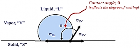
Young's equation provides the wettability of a flat surface, which is represented in Figure 1 by the contact angle (CA) of a water droplet. When gravitational forces can be ignored (often when the radius of the drop is smaller than the characteristic capillary length, which is approximately 2mm under ordinary conditions), it predicts the local contact angle of the edge of a droplet, according to Escandón-Panchana et al. [6].
Figure 1. Contact angle reflection
$\cos \theta=\frac{\gamma_{S G}-\gamma_{S L}}{\gamma_{L G}}$ (1)
where, θ is the local contact angle, $\gamma_{S G}$, $\gamma_{S G}$ and $\gamma_{S L}$ are the surface tensions of the solid-gas, solid-liquid, and liquid-gas interfaces. If the surface of the liquid is "wetted" or not depends on the local contact angle. A liquid is considered to be wetting if the local contact angle is less than 90o, and non-wetting if the local contact angle is more than 90o. In particular, a surface is referred to as "hydrophilic" if it is wetted by water and "hydrophobic" if it is not. From Michel and Fingas [7], this is illustrated in Figure 2. This contact angle controls a wide range of hydrodynamic phenomena, including the spontaneous spreading of the liquid over the surface, capillary action, and many others because Young's equation depicts the balance of forces exerted by surface tensions at the edge of the drop.
Only anisotropic, smooth surfaces are covered by the aforementioned equation. In their 2011 study, Nwilo and Badejo [8] employed a model based on Young's equation which considered surface roughness.
This model is known as the Cassie-Baxter equation:
$\cos \theta^*=r_f \cos \theta+f-1$ (2)
where, θ* is the composite surface's apparent water contact angle, f represents the percentage of the mesh coating's projection that is in touch with the liquid, and rf is the roughness ratio of the portion of the mesh coating that is wet by the liquid (ratio of actual surface area to apparent surface area). θ is the contact angle of water on a smooth coated surface. It should be noted that the apparent contact angle increases for surfaces that are hydrophobic (θ > 90°) and decreases for surfaces that are hydrophilic by increasing the roughness ratio. Additionally, since the contact angle of any liquid with air is believed to be 180o, decreasing the fraction of solid in contact with the liquid will increase the apparent contact angle for any type of surface. This amount of air has an impact on the value of f that passes through the mesh holes and any partial coating of the coated surface brought on by insufficient wetting of submicron structures. It is significant to note that Low-Density Polyethylene (LDPE) was utilized as the mesh coating in the aforementioned work. A cross-section of the water meniscus suspended with an idealized coated mesh hole is shown in Figure 3.
Figure 2. Hydrophilic and hydrophobic wetting
Figure 3. Cross-section of the water meniscus suspended within an idealized coated mesh aperture [3]
The contact point (represented by the angle from the horizontal, φ) moves up or down the surface of the wire while keeping a constant contact angle θ in relation to the local tangent as the water column height above the meniscus changes [9].
1.2 Surface roughness
The degree of surface roughness has a large impact on how well a surface repels liquid. Superhydrophobic surfaces typically have micro- or nanoscale asperities (rough). The behaviour of a water droplet on a rough surface is schematically depicted in Figure 4.
Figure 4. A liquid drop's behaviour on a rough surface. The liquid penetrates the spikes (Denzel state) on the left, and the liquid suspends on the spikes (right) (Cassie-Baxter state)
Figure 4 depicts Wenzel's hypothesis, which is based on the fundamental assumption that liquid follows surface roughness (left). The actual surface area divided by the anticipated surface area yields the roughness factor, or rf, which, according to Eq. (2), is greater than 1. According to Wenzel's prediction $\theta^w>\theta>90^{\circ}$ for a hydrophilic surface and $\theta^w>\theta>90^{\circ}$ for a hydrophilic surface.
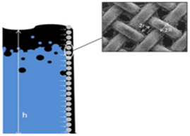
So far in this field of research, the parameter called Breakthrough Pressure has been a major limiting factor in the development of the hydrophobic-oleophilic mesh design. As defined by Abii and Nwosu [10], the Breakthrough water Pressure is the depth at which the capillary pressure inside the mesh holes is overcome by the hydrostatic water pressure. It is the maximum operation depth for a given mesh. Shown in Figure 5 is a pictorial representation of a hydrophobic mesh immersed at a depth of breakthrough pressure h.
Figure 5. Pictorial representation of a mesh in an oil-water medium immersed at breakthrough pressure depth h
In the course of this research, several procedures and methods were employed in the generation of results.
2.1 Materials selected
The simulation parameters for the hydrophobic mesh for oil spill remediation, the materials chosen, along with their properties for air are 1.225 kg/m3, 1.7894e-05 kg/m-s, 28.966 kg/kmol as the density of air, viscosity and molecular weight respectively. For Liquid water (H2O(l)), the respective values of density, viscosity and molecular weight are 998.2 kg/m3, 0.001003 kg/m-s and 18.0152 kg/kmol. For Liquid Fuel Oil (C19H3O(l)), the values for density, viscosity and molecular weight are 960 kg/m3, 0.048 kg/m-s, 258.19 kg/kmol respectively. The droplet surface tension is 0.032 N/m.
2.2 Fluid flow models
Several fluid flow models embedded in ANSYS Fluent for computational fluid dynamics were used in the simulation The models chosen, their governing equations, and the justifications for choosing them are discussed below:
2.2.1 Volume of Fluid (VoF) multiphase model
The VoF model can model two or more immiscible fluids by attempting to solve a single set of momentum equations and monitoring the volume fraction of each fluid throughout the domain. Examples of typical applications include the prediction of a jet breakup, the motion of large bubbles in a liquid, the flow of liquid after a dam break, and the steady or transient tracking of any liquid-gas interface.
This model was used to simulate the flow of air, water, and fuel-oil mixture. In this model, the three immiscible liquids are represented by air, water, and fuel oil. Thus, the three Eulerian phases mentioned above were selected for this flow simulation. It should also be noted that implicit body force formulation was used for this simulation to ensure the most accurate results. Accuracy of the implicit body force formulation is higher than the explicit body force because it improves solution convergence by accounting for the partial equilibrium of the pressure gradient and the body forces.
It should also be noted that the VoF multiphase model was used alongside the Viscous Laminar model. This is because the fluid flow occurs in the laminar region: Reynold’s number < 2000. It should also be noted that Implicit Volume Fraction Parameters were employed since this can be used for steady-state calculations, the governing Equations is presented in Eq. (3):
Volume Fraction Equation for Implicit Formulation Discretization:
$\frac{\alpha_q^{n+1} \rho_q^{n+1}-\alpha_q^n \rho_q^n}{\Delta t} V+\sum_f\left(\rho_q^{n+1} U_f^{n+1} \alpha_{q \cdot f}^{n+1}\right)=\left[S_{\alpha q}+\sum_{p=1}^n\left(m_{p q}^{\prime}-m_{q p}^{\prime}\right)\right]$ (3)
where:
n+1 = Current time step index
n= the preceding time step's index
$\alpha_q^{n+1}$ = volume fraction's cell value at time step n+1
$\alpha_q^{n}$ = volume fraction in the cell at time step n
$\rho_q^{n+1}$ = face value of volume fraction at time step n+1
$\rho_q^{n}$ = face value of volume fraction at time step n
$U_f^{n+1}$ = volume flux through the face at time step n+1
V = cell volume
Solving the momentum equation below throughout the domain, then the resulting velocity field is distributed among the phases. Through the properties ρ and μ, the momentum Eq. (4) is a function of the volume fractions of all phases.
$\frac{\partial}{\partial t}(\rho \vec{v})+\nabla \cdot(\rho \vec{v} \vec{v})=-\nabla \rho+\nabla \cdot\left[\mu\left(\nabla \vec{v}+\nabla \vec{v}^T\right)\right]+\rho \vec{g}+\vec{F}$ (4)
where:
$\rho$ = fluid density (kg/m3)
$\vec{v}$ = fluid velocity (nm/s)
$\vec{g}$= gravitational acceleration (m/s2)
$\vec{F}$= Force (N)
$\mu$ = viscosity (kg/m-s)
2.2.2 Surface tension and wall adhesion model
Surface tension is caused by the attractive forces that exist between molecules in a fluid. The VoF model takes into account surface tension as well as the interface between each pair of phases. Additional contact angle specifications between the phases and the walls were added to this surface tension model. The coefficients of surface tension were also specified as constants. For modelling flow across a hydrophobic medium, the following values of parameters were meticulously arrived at, surface tension for water-air, oil-air and oil-water interfaces are 0.072, 0.032 and 0.050 N/m respectively while the respective values of contact angle for water-air, oil-air and oil-water interfaces are 155o, 0.05o, and 1o.
Governing equations:
We made use of the Continuum Surface Force (CSF) model in ANSYS Fluent as proposed by Oladejo et al. [11]. The general mathematical representation of the Continuous Surface Force (CSV) model is given by
$p_2-p_1=\sigma\left(\frac{1}{R_1}+\frac{1}{R_2}\right)$ (5a)
The following Eq. (5b) was employed in determining pressure drop across surfaces
$p_2-p_1=\gamma\left(\frac{1}{R_1}+\frac{1}{R_2}\right)$ (5b)
where,
γ = surface tension coefficient (N/m)
p2 and p1 are the fluid pressures on either side of the interface (N/m2)
R1 and R2 are Radii in orthogonal directions (m)
2.3 Flow domain geometry
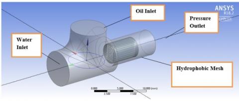
A flow domain model was developed for the hydrophobic-oleophilic mesh filled with oil and water. Visual representations of this flow domain are given in Figure 6. The dimension of the component is 1×1 m2 and the material used is stainless steel.
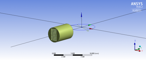
The hydrophobic mesh was placed in the path of fluid flow in such a manner that ensures that the fuel oil is filtered out by it. The geometry for the hydrophobic mesh is given in Figure 7.
In Figure 7, each mesh square opening has a dimension of 334e-06m × 334e-06m [12-15]. The flow domain generated allows for an interface between the oil and water phases. This was an attempt to simulate the interfacial conditions that occur during an oil spill, seeing that oil floats on water (because of the density of oil< density of water).
Figure 6. Orthographic view of flow domain
Figure 7. Geometric representation of a hydrophobic mesh
2.4 Domain discretization (Meshing)
The flow domains are discretized into smaller subdomains made up of geometric primitives to analyze the fluid flow as depicted in Figure 8. Inside these subdomains, the governing equations are discretized and solved
Figure 8. Visual representation of domain discretization
2.5 Discretization parameters
Discretization details are given below:
Element Order: Linear
Size Function: Curvature
Maximum Face Size: Default (3.7025e-004 m)
Mesh Defeaturing: Yes
Defeature Size: Default (1.8513e-006 m)
Transition: Slow
Growth Rate: Default (1.20)
Span Angle Centre: Fine
Minimum Size: Default (3.725e-006 m)
Maximum Tet Size: Default (7.4051e-004 m)
Curvature Normal Angle: Default (18.0°)
Bounding Box Diagonal: 2.5362e-002 m
Minimum Edge Length: 3.34e-004 m
Target Skewness: Default (0.900000)
Smoothing: High
Inflation Option: Smooth Transition
Transition Ratio: 0.272
Maximum Layers: 5
Growth Rate: 1.2
Inflation Algorithm: Pre
Pinch Tolerance: 3.3323e-006 m
Number of Nodes: 18375
Number of Elements: 79734
2.6 Solution setup
For the simulation, a pressure-based solver was chosen. This is due to the VoF model's reliance on a pressure-based solver. Steady-state conditions were also assumed. This is because the final state of the system is of utmost importance. Furthermore, a gravitational constant of 9.81 m/s2 was applied in the negative z-direction.
As previously stated, the Multiphase VoF model was chosen. Surface tension and wall adhesion models in the VoF model were enabled to input interfacial tension values. The Viscous Laminar model was activated in addition to the VoF model. It should be noted that air was designated as the primary phase, with water and oil designated as the secondary phases. Primary phases are continuous phases while secondary phases are dispersed.
Three phases, Water, Fuel-oil, and Air, were selected from the fluent materials database.
Cell zone conditions were kept as fluid for both flow domain geometry and hydrophobic mesh domain.
2.6.1 Boundary conditions
1. Oil Inlet: This was set as a velocity inlet. The magnitude of the velocity was set to 0.1 m/s, while the supersonic/initial gauge pressure (pascal) was set to zero. The volume fraction of oil was set to 1, while the volume fraction of water was left at zero. Shown in Figure 13 is a pictorial representation of the oil inlet boundary.
2. Water Inlet: This was set as a velocity inlet. The velocity magnitude was set to 0.1 m/s, while the supersonic/initial gauge pressure (pascal) was set to zero. The volume fraction of water was set to 1, while the volume fraction of oil was left at zero. Figure 14 is a pictorial representation of the water inlet boundary.
3. Outlet: This was configured as a pressure outlet with a gauge pressure of 0 Pascal (atmospheric pressure).
Interior-part-solid-mesh: this describes the boundary between the hydrophobic mesh and the interior of the flow domain geometry. This was set to “wall” to set appropriate contact angles at interface boundaries. At the “wall”, the fluid velocity is zero and the viscosity is zero – a no-slip condition.
Factors relating to setting of contact angle are surface roughness, particle shape and size, heterogeneity and temperature. Wall motion was set to “Stationary Wall” with “No Slip” boundary conditions. Appropriate contact angles were set as discussed previously. The operating density was set to 1.225 kg/m3, which is the primary phase-Air density.
2.6.2 Solution methods
SIMPLEC (Semi-Implicit Method for Pressure Linked Equations-Consistent) was chosen as the solution method. The specific process for implementation of SIMPLEC is as follows:
- START
- Solve discretized momentum equation
- Solve Pressure Correction equation
- Correct pressure and velocities
- Check for convergence
- STOP
This is due to the SIMPLEC skewness correction, which allows a solution to be obtained on a highly skewed mesh in roughly the same number of iterations as a more orthogonal mesh. Skewness correction was set to 0. Hybrid initialization was then carried out with 20 iterations, after which a value of 4.486648e-07 was reached. Patching was also done for both secondary phases. The calculation was then run for 350 iterations.
The results for the steady-state, three-dimensional flow of oil-water flow through a hydrophobic porous medium with a thickness of 55mm and mesh opening of 0.334mm × 0.334mm were obtained numerically. The mesh number was determined by the version of ANSYS we used for the work – which is the Students’ version.
The governing equations of the model given in section 2 are valid for 1D, 2D and 3D. However, the numerical implementation presented in this work is only in 3D. This is to allow for more robust illustrations of solutions.
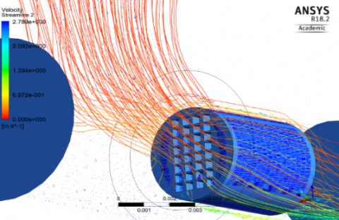
3.1 Velocity streamlines
In Figure 9, the fluid flow of both the oil and water phase in the flow domain across the Hydrophobic Mesh is shown. It is observed that for the water phase (coloured blue), the streamlines do not pass through the mesh (as is properly shown in Figure 10), while the oil phase is permitted to pass through the mesh (as is more clearly illustrated in Figure 11).
Figure 9. Illustration of 2-Phase velocity streamlines
Figure 10. Illustration of water phase velocity streamlines
Figure 11. Illustration of oil phase velocity streamlines
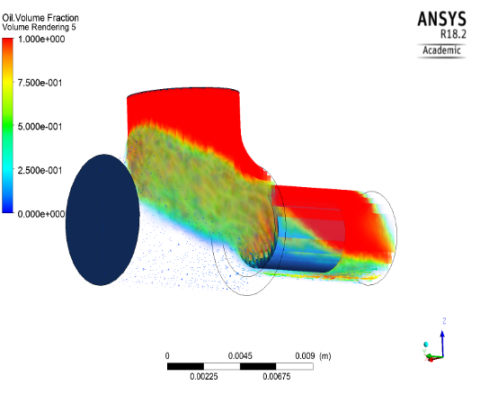
3.2 Volume fraction
Shown in Table 1 are the volume fractions for each phase in the flow domain.
Table 1. Volume fraction per phase
|
Phase |
Volume fraction |
|
Air |
0.006904962 |
|
Water |
0.4843525 |
|
Oil |
0.50874251 |
Pictorial representations of both the oil and water phase volume fraction through the flow domain and across the Hydrophobic Mesh are shown in Figures 12 and 13 respectively.
Figure 12. Pictorial representation of oil volume fraction
Figure 13. Pictorial representation of water volume fraction
3.3 Static pressure per zone
Given in Table 2 below are the calculated static pressures per zone in the flow domain.
Table 2. Static pressure per zone
|
Zone |
Static Pressure (pascal)(kg/s) |
|
Interior part solid |
-107.47672 |
|
Interior part solid porous medium |
0 |
|
Interior part solid porous medium shadow |
0 |
|
Interior porous medium |
2.6500401e-11 |
|
Oil inlet |
22.832333 |
|
Outlet |
0.0092529729 |
|
Wall part solid |
0 |
|
Water inlet |
23.921438 |
|
Net |
-60.713699 |
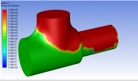
3.4 Phase contours
Phase contours depict a general overview of the fluid flow during the entirety of the process. This shows the behaviour of immiscibility of the oil and water phases [16, 17]. A pictorial representation of the Phase contours for Oil and Water during the flow process is given below in Figure 14.
Figure 14. A pictorial representation of phase contours during fluid flow
It should be noted that the green contours represent the water phase, while the red contours represent the oil phase.
3.5 Mass flow rate
Table 3. Mass flow rates for oil phase per zone
|
Zone |
Mass Flow Rate (kg/s) |
|
Oil inlet |
0.0036675623 |
|
Outlet |
-0.004020479 |
|
Interior-part-solid |
-0.012882997 |
|
Interior-porous medium |
-1.3935695e-14 |
|
Net |
-0.013235914 |
Table 4. Mass flow rates per zone for water phase
|
Zone |
Mass Flow Rate (kg/s) |
|
Water inlet |
0.0038135007 |
|
Outlet |
0.0032380666 |
|
interior-part-solid |
-0.027856153 |
|
interior-porous medium |
-1.4490221e-14 |
|
Net |
-0.027280718 |
Deduced from calculations run by the simulation are the mass flow rates for both the oil and water phase per zone in the flow domain. Mass flow rates are not affected by change in pressures and temperatures [18, 19]. Characteristics of oil and water are not subjected to variations in temperatures and pressure.
This serves as a guide in the measurement of the effectiveness of the proposed Hydrophobic Mesh for oil-water separation [20]. Given in Tables 3 and 4 are the mass flow rates per zone for both the oil and water phase respectively.
From the results gotten above, it is observed that the use of Hydrophobic Mesh for Oil Spill remediation -with further research- is largely feasible.
4.1 Conclusions
In conclusion, the project research and simulation were successfully carried out. Properties of hydrophobic-oleophilic coatings were employed in this simulation. Appropriate selection of Hydrophobic Mesh parameters was also done in the course of this project.
Furthermore, diverse parameters and equations were employed for the development of the hydrophobic mesh simulation. The finite element analysis was also successfully simulated in ANSYS Fluent environment.
This research has proven to be a step forward in the industrialization of the use of hydrophobic mesh for oil spill clean-up.
4.2 Future works
It is recommended that for future work in this field, computers with high computing powers and processing speeds be employed, to be able to study transient conditions.
Also, it is recommended that ANSYS Student Version should NOT be used for future work in this area. Rather, ANSYS Professional package should be employed. This will permit more complex geometry designs, even to the level of microstructures.
[1] Brackbill, J.U., Kothe, D.B., Zemach, C. (1992). A continuum method for modeling surface tension. Journal of Computational Physics, 100(2): 335-354. https://doi.org/10.1016/0021-9991(92)90240-Y
[2] Button, S.T. (2000). Numerical simulation and physical modeling as educational tools to teach metal forming processes. In ICECE 2000–International Conference on Engineering and Computer Education, 27-30. http://copec.eu/congresses/icece2000/proc/papers/034.pdf.
[3] Cassie, A.B.D. (1944). Discussions Faraday Soc., 3 (1948) 11. ABD; Cassie and S. Baxter. Transactions of The Faraday Society, 40: 456-456.
[4] Coene, E., Silva, O., Molinero, J. (2018). A numerical model for the performance assessment of hydrophobic meshes used for oil spill recovery. International Journal of Multiphase Flow, 99: 246-256. https://doi.org/10.1016/j.ijmultiphaseflow.2017.10.011
[5] Deng, D., Prendergast, D.P., MacFarlane, J., Bagatin, R., Stellacci, F., Gschwend, P.M. (2013). Hydrophobic meshes for oil spill recovery devices. ACS Applied Materials & Interfaces, 5(3): 774-781. https://doi.org/10.1021/am302338x
[6] Escandón-Panchana, P., Morante-Carballo, F., Herrera-Franco, G., Rodríguez, H., Carvajal, F. (2022). Fluid level measurement system in oil storage. Python, Lab-based scale. Mathematical Modelling of Engineering Problems, 9(3): 787-795. https://doi.org/10.18280/mmep.090327
[7] Michel, J., Fingas, M. (2016). Oil Spills: Causes, consequences, prevention, and countermeasures. In Fossil fuels: Current Status and Future Directions, 159-201. https://doi.org/10.1142/9789814699983_0007
[8] Nwilo, P.C., Badejo, O.T. (2006). Impacts and management of oil spill pollution along the Nigerian coastal areas. Administering Marine Spaces: International Issues, 119: 1-15.
[9] Nwilo, P.C., Badejo, O.T. (2004). Management of oil spill dispersal along the Nigerian coastal areas. Department of Surveying and Geoinformatics, University of Lagos. http://hdl.handle.net/1834/267.
[10] Abii, T.A., Nwosu, P.C. (2009). The effect of oil-spillage on the soil of eleme in rivers state of the niger-delta area of nigeria. Research Journal of Environmental Sciences, 3(3): 316-320. https://doi.org/10.3923/rjes.2009.316.320
[11] Oladejo, K.A., Abu, R., Adewale, M. (2012). Effective modeling and simulation of engineering problems with COMSOL Multiphysics. International Journal of Science and Technology, 2(10): 742-748.
[12] Prendergast, D.P. (2013). Optimization of hydrophobic meshes for oil spill recovery. Doctoral dissertation, Massachusetts Institute of Technology. http://hdl.handle.net/1721.1/82848
[13] Prendergast, D.P., Gschwend, P.M. (2014). Assessing the performance and cost of oil spill remediation technologies. Journal of Cleaner Production, 78: 233-242. https://doi.org/10.1016/j.jclepro.2014.04.054
[14] Prendergast, D.P. (2013). Optimization of hydrophobic meshes for oil spill recovery. Doctoral dissertation, Massachusetts Institute of Technology.
[15] Simpson, J.T., Hunter, S.R., Aytug, T. (2015). Superhydrophobic materials and coatings: A review. Reports on Progress in Physics, 78(8): 086501. https://doi.org/10.1088/0034-4885/78/8/086501
[16] Song, J., Huang, S., Lu, Y., Bu, X., Mates, J. E., Ghosh, A. (2014). Self-driven one-step oil removal from oil spill on water via selective-wettability steel mesh. ACS Applied Materials & Interfaces, 6(22): 19858-19865. https://doi.org/10.1021/am505254j
[17] Spyrakos, C. (1994). Finite element analysis in engineering practise. West Virginia University Press, USA.
[18] Moore, I.D., Mississippi, J. (1981). Water Resour. Resources, 23(8): 1514-1522.
[19] Li, X.M., Reinhoudt, D., Crego-Calama, M. (2007). What do we need for a superhydrophobic surface? A review on the recent progress in the preparation of superhydrophobic surfaces. Chemical Society Reviews, 36(8): 1350-1368. https://doi.org/10.1039/B602486F
[20] Rahman, F., Sugiono, S., Sonief, A.A., Novareza, O. (2022). Availability optimization of the mobile crane using approach reliability engineering at oil and gas company. Mathematical Modelling of Engineering Problems, 9(1): 178-185. https://doi.org/10.18280/mmep.090122