Albio D. Gutierrez* | Luis F. Alvarez
© 2022 IIETA. This article is published by IIETA and is licensed under the CC BY 4.0 license (http://creativecommons.org/licenses/by/4.0/).
OPEN ACCESS
This work presents a simplified methodology to couple the physics of a nanosecond pulsed discharge to the process of supersonic combustion in a flat wall combustor configuration. Plasma and supersonic combustion are separately simulated and then coupled by seeding plasma-generated radicals on the combustion domain. The plasma model is built assuming spatial uniformity and considering only the kinetic effects of the nanosecond pulsed discharge. Therefore, a zero-dimensional kinetic scheme accounting for the generation of plasma species is utilized. For the combustion model, the complete set of Favre-averaged compressible Navier Stokes equations along with finite rate chemistry is solved through a control-volume based technique via the commercial software Ansys Fluent. The computational results are compared against experimental studies showing that the proposed methodology can capture the main kinetic effects of the nanosecond pulsed discharge on supersonic combustion. OH concentration contours reveal the presence of an enhanced flame when the plasma is applied following the trends from experimental OH PLIF images. In addition, time evolving temperature and OH concentration contours show that the ignition delay time is reduced with the application of the discharge.
supersonic combustion, plasma-assisted combustion, nanosecond pulsed discharge, scramjet
Over the last decades, there have been an increasing interest in hypersonic vehicles due to their capability in enabling low-Earth orbit flights and defense and transport applications [1-7]. The scramjet engine is a candidate for this type of applications. These engines burn substantial amounts of fuel to generate the thrust necessary to achieve hypersonic velocities. Efficient combustion of fuel is one of the technical challenges faced by scramjets [8].
At speeds above Mach 7 inside the scramjet engine, the flow residence time is shorter than the ignition delay time and the fuel consumption time of typical mixtures. Hence, the fuel-air mixture does not have enough time to autoignite and burn completely. This gives way to inefficient fuel use, and therefore, the flow may not achieve a faster speed than the incoming air.
Different methods have been proposed to tackle the challenge of the short flow residence time for mixing and igniting. This includes radical addition, temperature and pressure increase at the combustor inlet via shockwaves, changing the fuel/oxidizer mixtures and mixing enhancement [9, 10]. The problem of holding and stabilizing the flame has been approached with different techniques, such as adding bluff bodies as fuel injectors that block the flow and increase mixing through vortex generation [11-13]. Another alternative is normal supersonic fuel injection, which generates bow shocks, leading to subsonic regions that promote mixing [14], [15]. Furthermore, cavities and steps have been used as flame holders, generating recirculation zones that allow the air and fuel to mix more slowly and increase the flow residence time in the combustor of the scramjet engine [16-21].
Despite that all the aforementioned strategies improve combustion through shorter ignition times, increased mixing, longer residence times and increased flame holding, they are still static and difficult to optimize for the entire range of scramjet flight conditions, such as altitude, velocity, pressure and incoming air temperature. In addition, geometric alterations can induce shockwaves in the combustor which lead to stagnation pressure losses that increase as the flight Mach number increases [22, 23].
Lately, as an alternative method in supersonic combustion, plasma-assisted combustion (PAC) has shown remarkable capabilities in improving fuel/air mixing, ignition and flame stabilization. The enhancement of supersonic combustion by PAC can be classified as kinetical [24-30], thermal [31-35], and plasma-induced aerodynamic effects [36-38]. Nonequilibrium plasmas, such as corona microwave, low-pressure glow, and nanosecond high-voltage discharges improve combustion by adding active radicals leading to the modification of chemical reaction pathways and therefore combustion times are shortened [27]. Experimental studies in these types of plasmas have shown that the introduction of radicals reduces the ignition delay time and kinetically enhances flame stability in supersonic environments [39]. However, in-ground flight testing of supersonic combustors has financial and technical difficulties, leading to limited test conditions. Furthermore, the capability of ground facilities is insufficient for reproducing all the conditions describing the scramjet flow field for full-scale engines such as matching enthalpy and Mach numbers [40]. Hence, computational models and analysis are required to obtain an in-depth understanding of the phenomenon of plasma in scramjet engines and to perform rapid tests of different geometric designs and test conditions. Simulations and experiments complement each other. PAC in supersonic flows can be simulated using both detailed and simplified models. Detailed models include the full coupling of plasma physics with supersonic combustion flows, which implies a high computational burden. Simplified plasma modeling, however, focuses on the most representative plasma effects on combustion, according to the type of discharge simulated. Kinetics effects are dominant for nanosecond pulsed discharges, which were used in this work.
PAC detail modeling includes fully-coupled plasma-combustion chemistry and sets of stiff equations representing generation and transport of plasma species, plasma-induced heat and electromagnetic forces [41]. Some of these models also include Large Eddy Simulations (LES) for turbulence modeling [42]. Despite the details of these PAC models, certain studies have shown that plasma effects on combustion, such as heating, electromagnetic forces and current densities, are lower than kinetic effects in nanosecond-plasma discharges [43-46]. Furthermore, it has been shown by some studies [47, 48] that H and O radicals generated by the plasma are mainly responsible for reducing the ignition delay time. For instance, Bozhenkov et al. [47] studied the kinetics of plasma-combustion applying a nanosecond plasma discharge in a shock tube. The experiment was innovative in separating the thermal plasma effect from the kinetic effect. It was shown that the plasma kinetic effect can lead to a decrease of the H2 ignition delay time by almost one order of magnitude. This ignition delay was primarily a result of H and O produced during the discharge.
These previous findings have been used by authors such as Do et al. [39] to develop simplified models assuming constant plasma parameters, including electric fields and gas density, while neglecting heat and magnetic contributions, as well as certain plasma reactions, for nonequilibrium discharges. Given that nanosecond-pulsed plasmas mostly lead to the production of radicals to initiate combustion reactions, Do et al. [39] neglected excited and ionized species generation and utilized a simplified radical yield calculation method for dissociation reactions in a H2-O2 mixture. The model also neglected heat and plasma aerodynamic effects.
Whereas these simple plasma models do not predict aspects such as charged species transport or thermal or aerodynamic plasma effects, the results regarding radical generation are quite logical according to combustion enhancement experiments [39, 49-51]. In addition, different time and length scales for nonequilibrium plasmas and supersonic flows allow for additional model simplifications [41, 43], leading to results that are relatively close to experiments.
Detailed models require expensive computations to assembly the Poisson’s Equation with the electron density and energy equations. Simplified models, on the other hand, eliminate these demanding calculations by making the aforementioned assumptions. This minimized complexity of the simplified models for nanosecond-plasma discharges is mainly due to assumptions that lead to equations that account for kinetic plasma effects while neglecting thermal and magnetic effects on combustion. However, current simplified models, such as that of Do et al. [39, 49], ignore important flow effects such as turbulence, fuel-oxidant mixing and compressibility. All these factors are critical in supersonic combustion and therefore influence PAC models. Although it is possible to simplify the detailed chemical and electrical properties of the plasma when modeling nonequilibrium discharges, it is also important to include turbulence and compressible flow effects in these simplified models. Hence, the computational demand decreases in terms of plasma modeling. To sum up, reduced-order models that capture plasma-enhanced combustion as well as fluid flow and thermal transport at supersonic speeds could potentially reduce the computational cost involved in scramjet engine design.
Breden and Raja [41] and Do [49] have provided an opportunity to develop a model that simplifies the computationally expensive terms in plasma models while including the effects of combustion, turbulence and compressibility of supersonic reacting flows.
According to previous results, this work, unlike detailed plasma-assisted combustion models in the literature, proposes a simplified methodology for simulating plasma in supersonic combustion by separating plasma kinetics from combustion kinetics and coupling the plasma and reacting flow phenomena solely by cyclically seeding O and H radicals into the computational flow domain. Furthermore, while some simplified plasma combustion models calculate only the plasma radical yield via short-cut estimations while ignoring mixing, turbulence and shock wave flow effects on combustion, the model proposed in this study solves plasma kinetics for a variety of species and calculates supersonic reacting flow patterns for compressible turbulence flows via CFD, resulting in more accurate results.
Additionally, the PAC supersonic combustion experiment from Do et al. [51] was simulated in great detail. Other works have performed simulations of this experiment without decoupling the combustion kinetics from the plasma kinetics, with LES turbulence model and with no direct comparison to experimental results and they are not focused on studying the ignition effect of the plasma. In this work, on the other hand, the proposed methodology is applied to simulate the experiment, decoupling the combustion from plasma kinetics, and some computational results from ignition are compared with experimental results.
The governing equations for the nanosecond plasma discharge and the supersonic combustion phenomena are separately solved and their results are subsequently coupled. This separation was made based on two facts. First, the effect of the plasma on reducing the ignition delay time is mainly due to the radicals produced by the discharge according to the study of Bozhenkov in shock tubes [47] and therefore kinetic effects are more significant than thermal and electromagnetic effects. Second, the nanosecond pulse discharge and the compressible reactive flow processes have different characteristic time scales. The nanosecond-pulsed plasma discharge simulation occurs on a nanosecond scale, in which radicals are generated, whereas the time-step size of the compressible reactive flow is characterized by the Courant number criteria, which is 1.2 x 10⁻⁸ s in this case. The time size step for the discharge simulation was set to 5 x 10⁻¹⁰ s. Therefore, one discharge pulse is shorter than a single reactive flow step. This fact also allows us to separate the plasma chemistry from the combustion chemistry.
For the plasma-flow coupling approach, it is assumed that effect of the discharge is reduced to the seeding of O and H radicals produced by the plasma into the combustion environment having a significant impact on ignition [47]. In addition, the plasma model considers the discharge to be spatially uniform, which will be explained in Section 2.1.2. Based on this assumption, the plasma radicals are assumed to be concentrated uniformly during each electric discharge pulse only in the region of the computational combustion domain formed by the electric discharge electrodes that represent the plasma volume. Therefore, O and H radicals are uniformly seeded in this area.
The equations modeling the physics of the unsteady turbulent compressible reactive flow are solved using Ansys Fluent and the plasma modeling equations are solved using ZDPlaskin [52] and Bolsig+ [53] software.
The proposed plasma and reacting flow modeling approaches are coupled as follows. For each flow step the Fluent solver updates the species concentration, pressure, temperature, velocity fields and turbulence information. For each plasma pulse, the area-average flow data calculated in the area of the discharge is used as input by the plasma kinetics solver to compute the plasma species densities. Subsequently, the density of the O and H radicals produced during the discharge is seeded on the discharge area inside the computational domain of the combustion simulation to update again the flow parameters in the new flow step. Figure 1 shows that the entire process is a cycle. The plasma solver needs information about the pressure, temperature and gas composition of the gas in order for Bolsig+ to calculate the reaction rate coefficients and subsequently obtain the plasma concentration. Similarly, the flow solver requires the plasma-generated species information to calculate the combustion reactions and update the flow parameters.
Figure 1. Schematic of plasma-flow coupling cycle
Unlike detailed plasma assisted combustion models in the literature, the current approach provides a simplified methodology to simulate plasma in supersonic combustion by separating plasma kinetics from combustion kinetics and coupling plasma and reacting flow phenomena solely by seeding O and H radicals into the computational flow domain cyclically. Furthermore, while certain simplified plasmas combustion models calculate only the plasma radicals yield via short-cut estimations and avoids mixing, turbulence and shock waves flow effects on combustion, the model proposed in this study solves the plasma kinetics for a variety of species and calculates supersonic reacting flow patterns for compressible turbulence flows via CFD so more accurate results can be obtained.
2.1 Governing equations
2.1.1 Compressible reacting flow model
Ansys Fluent was used for the simulations in this work. In order to model the reactive compressible flow in the flat wall, a density-based approach was selected on Ansys Fluent which models the density using the ideal gas law. Concerning turbulence modeling, the Favre-averaged mean mass, momentum and energy conservation equations were considered which accounts for density variations. These averaged equations are shown in (1), (2) and (3), respectively, describing the turbulent, supersonic, unsteady, viscous and thermally perfect flow inside a scramjet combustor. The correlations of the fluctuating terms in these equations are analyzed using the k-ε renormalization group, RNG [54]. In Eqns. (1)-(6). $\bar{\rho}$ is the Reynolds-averaged density, $\tilde{u}_t$ is the Favre-averaged velocity vector in i direction, xi is the distance in i direction, $\widetilde{u_k}$ is the Favre-averaged velocity vector in k direction, $\tilde{u_J}$ is the Favre-averaged velocity vector in j direction, xj is the distance in j direction, t is the time, P is the static pressure, $\bar{\tau}_{j i}$ is the averaged viscous shear stress tensor, uj'' is the fluctuating-Favre velocity vector in j direction, ui'' is the fluctuating-Favre velocity vector in i direction E is the total energy, H is the total enthalpy, Keff id the thermal conductivity, $\tilde{T}$ is the Favre-averaged temperature $\tilde{h}_n$ is the sensible enthalpy of species n, Jn,j is the diffusion flux of species n in direction j, h'' is the fluctuating-Favre enthalpy, $\tilde{e}$ is the Favre-averaged internal energy and k is the turbulence kinetic energy.
$\frac{\partial \bar{\rho}}{\partial t}+\frac{\partial\left(\bar{\rho} \widetilde{u_l}\right)}{\partial x_i}=0$ (1)
$\frac{\partial\left(\bar{\rho} \widetilde{u_k}\right)}{\partial t}+\frac{\partial\left(\bar{\rho} \widetilde{u_{\imath}} \widetilde{u_J}\right)}{\partial x_j}=-\frac{\partial P}{\partial x_i}+\frac{\partial}{\partial x_j}\left(\bar{\tau}_{j i}-\overline{\rho u_j^{\prime \prime} u_{\imath}^{\prime \prime}}\right)$ (2)
$\frac{\partial(\bar{\rho} \mathrm{E})}{\partial t}+\frac{\partial\left(\bar{\rho}{\widetilde{u_j}}^H\right)}{\partial x_j}=\frac{\partial}{\partial x_j}\left[K_{e f f} \frac{\partial \tilde{T}}{\partial x_j}-\sum_n \tilde{h}_n J_{n, j}-\overline{\rho u_j^{\prime \prime} h^{\prime \prime}}+\right.
\left.\overline{\bar{\tau}_{j l} u_{\imath}^{\prime \prime}}-\frac{\overline{\rho u_{\jmath^{\prime \prime}} u_{l^{\prime \prime}} u_{l^{\prime \prime}}}}{2}+\tilde{u}_{\imath}\left(\bar{\tau}_{j i}-\overline{\rho u_{\jmath}^{\prime \prime} u_{\imath}^{\prime \prime}}\right)\right]$ (3)
$E=\tilde{e}+\frac{\widetilde{u_l} \widetilde{u_l}}{2}+k$ (4)
$H=\tilde{h}+\frac{\widetilde{u_l} \widetilde{u_l}}{2}+k$ (5)
$\bar{\rho}=\frac{P_{o p}+P}{\frac{R}{M_W} \widetilde{T}}$ (6)
The ideal gas law was utilized to model the density of the mixture, as shown in Eq. (6), where Pop is the operating pressure, R is the universal gas constant and MW is the molecular weight.
The mixing and transport processes of the chemical species resulting from combustion were modeled by solving conservation equations for the local mass fractions of each species, as shown in Eq. (7). In this equation, Eq. (8) Yn is the local mass fraction of species n, $\vec{J}_n$ is diffusion flux of species n, Rn is the net rate of production of species n by chemical reactions, Dn,m is the binary diffusion of species n in each species m, μt is the turbulent dynamic viscosity, Sct is the turbulent Schmidt number and DT,n is the thermal diffusion of species n.
Eq. (9) combines Eqns. (3) and (7) to model the enthalpy contribution of each species to energy conservation, where h enthalpy of the mixture and hn is the sensible enthalpy of species n. Eq. (10) shows that this enthalpy contribution depends on both the temperature and the specific heat of each species, cp,n.
$\frac{\partial\left(\rho Y_n\right)}{\partial t}+\frac{\partial\left(\rho u_i Y_n\right)}{\partial x_i}=-\nabla \cdot \vec{J}_n+R_n$ (7)
$\vec{J}_n=-\left(\rho D_{n, m}+\frac{\mu_t}{S c_t}\right) \frac{\partial Y_n}{\partial x_i}-D_{T, n} \frac{1}{T} \frac{\partial \mathrm{T}}{\partial x_i}$ (8)
$h=\sum_j Y_n h_n$ (9)
$h_n=\int_{T r e f}^T c_{p, n} d T$ (10)
To account for the production of chemical species from combustion reactions, the second term on the right-hand side of Eq. (7), Rn, was defined according to the laminar finite rate model described in Eqns. (11), (12) and (13), where MW,n is the molecular weight of species n, NR is the total number of reactions in the system, $\widehat{R_{n, r}}$ is the Arrhenius molar rate of creation/destruction of species n in reaction r, $v_{n, r}^{\prime}$ is the stoichiometry coefficient for reactant n in reaction r, $\mathcal{M}_n$ is the symbol denoting species n, kfr is the forward rate constant for reaction r, $v_{n, r}^{\prime \prime}$ is the stoichiometry coefficient for product n in reaction r, Cm,r is the molar concentration of species m in reaction r, $\eta_{m, r}^{\prime}$ is the rate exponent for reactant species n in reaction r, $\eta_{m, r}^{\prime \prime}$ is the rate exponent for product species n in reaction r and $\Gamma_{t b}$ is the net effect of third bodies on the reaction rate. In the implemented reaction mechanisms, some reactions require a third species to generate the products. This third species does not chemically react but remove the excess energy from the reaction and dissipate it as heat. If a third species is required, its concentration must be indicated in order to calculate the rate of progress of that species. Some of these third species are more efficient than others in the reaction mechanisms. This contribution of each species as a third species in a reaction is modeled as third-body efficiencies.
The net effect of third bodies on the reactions rate were calculated according to Eq. (14) where γm,r is the third body efficiency of the mth species in the r th reaction. The reaction rates were determined via the Arrhenius law, as shown in Eq. (15) where Ar is the pre-exponential factor, βr is the temperature exponent, Ea,r is the activation energy for reaction r. Both third-body efficiencies and Arrhenius parameters were defined by the authors of the selected reaction mechanism [55]. This approach allowed for the calculation of multiple-step kinetic mechanisms, permitting the effect of active radicals on the chain-branching process to be captured. Radicals such as O, H and OH must react with other species to appropriately model combustion and plasma. Thus, multistep chemistry needs to be modeled over turbulent–chemistry interactions. While the reacting flow model presented in this work ignores the effect of turbulence on the production of species, supersonic flames are characterized by slower chemistry and smaller turbulence-chemistry interactions than subsonic flames [56].
$R_n=M_{W, n} \sum_{r=1}^{N_R} \widehat{R_{n, r}}$ (11)
$\sum_{i=1}^N v_{n, r}^{\prime} \mathcal{M}_n \stackrel{k f_r}{\rightarrow} \sum_{n=1}^N v_{n, r}^{\prime \prime} \mathcal{M}_n$ (12)
$\widehat{R_{n, r}}=\Gamma_{t b}\left(v_{n, r}^{\prime \prime}-v_{n, r}^{\prime}\right)\left(k f_r \prod_{m=1}^N\left[C_{m, r}\right]^{\left(\eta_{m, r}^{\prime}+\eta_{m, r}^{\prime \prime}\right)}\right)$ (13)
$\Gamma_{t b}=\sum_m^N \gamma_{m, r} C_m$ (14)
$k f_r=A_r T^{\beta_r} e^{\frac{-E_{a, r}}{R T}}$ (15)
The ideal gas mixing law was used to compute the viscosity of the mixture. The viscosity of each species in the mixture was modeled by the Sutherland law. The specific heat of each species in Eq. (10) was calculated as a function of the temperature via polynomials [56]. The mixture thermal conductivity K, required by the energy conservation equations was modeled according to Eq. (16) where Xn is the mole fraction of species n, kn is the thermal conductivity of the species n, Xm is the mole fraction of species m, ψnm is the function of the properties of pure components of the mixture. The mass, Dn,mix, and thermal, DT,n, diffusion coefficients in Eq. (8) were modeled according to Eqns. (17) and (18), respectively, whereas the turbulent diffusion coefficient was derived according to the turbulence model used [54].
$K=\sum_n \frac{X_n k_n}{\sum_m X_m \psi_{n m}}$ (16)
$D_{n, \operatorname{mix}}=\frac{1-n}{\sum_{n, m \neq n}\left(X_m / D_{n m}\right)}$ (17)
$D_{T, n}=-2.59 \times 10^{-7} T^{0.659} \mid \frac{M_{W, n}^{0.511} X_n}{\sum_{i=1}^N M_{W, n}^{0.511} X_n}-Y_n|| \frac{\sum_{n=1}^N M_{W, n}^{0.511} X_n}{\sum_{n=1}^N M_{W, n}^{0.489} X_n} \mid$ (18)
The system of equations was solved numerically by the k-ε RNG turbulence model using the commercial software ANSYS Fluent. The system of equations was discretized by a control-volume-based technique. Second-order upwind and least-squares cell-based schemes were utilized to discretize the convection and gradient terms, respectively. The density-based solver available was selected for the simulation [56].
2.1.2 Plasma model
Experimental Intensified Charge-Coupled Device (ICCD) camera images of nanosecond-pulsed discharges in air and hydrogen [57, 58] have shown that plasma is generated in an approximately rectangular, narrow shape near the lower wall, in the volume between the electrodes. In addition, it has been shown that the plasma is nearly uniform during each pulse. Starikovskaia et al. [59] also confirmed the uniformity of nanosecond-pulsed discharges in a gas mixture between 0.3 and 2.4 atm. Kosarev et al. [60] discussed the ability of these types of discharges to generate a quasi-uniform plasma layer behind a shock wave from a shock tube. As a result of these findings, certain studies for supersonic hydrogen-air mixtures [42, 50] have proposed modeling the plasma in a volumetric constant region with a uniform electric field throughout the domain. This approach reduces the computational load imposed by solving Poisson’s equation when computing electric fields and is utilized in this work to uniformly model the production of plasma active species in a constant volume between discharge electrodes. This is done by using a constant electric field derived from the discharge parameters.
Eq. (19) shows the plasma species transport, where nk is the number density of plasma species, Γk is the species k flux number and $\dot{G_k}$ is the plasma species k generation/destruction term. Due to the spatial uniformity of the plasma model in this work, the number density of the species produced during each pulse of the discharge is only a function of time. Thus, by eliminating the spatial transport term in Eq. (19), it is not necessary to solve the highly computationally-demanding electric potential equation. In addition, the current modeling approach does not consider the calculation of ion Joule heating because the energy contribution of this phenomenon is rapidly dissipated by convection. Finally, compared to electric fields, the current densities and induced magnetic fields are thought to have a minor impact on plasma physics of the nanosecond pulsed discharge [43].
$\frac{\partial n_k}{\partial t}+\nabla \cdot \Gamma_k=\dot{G_k}, \quad k=1,2,3$ (19)
As a result of the aforementioned assumptions, the plasma modeling approach used in this work calculates the concentrations of species generated during the application of an electric discharge solely as a function of time as shown in Eq. (20), where Qkm are the source terms for the species k corresponding to the contributions from different plasma reactions m. This gives way to a system of nonlinear ordinary differential equations as shown in Eqns. (21), (22) and (23) where Rpm is the reaction rate of plasma species and kpm is the plasma reaction rate coefficient. This approach allows to save computational resources while still capturing its main effects.
$\frac{d n_k}{d t}=\sum_{m=1}^m Q_{k m}(t)$ (20)
$a A+b B \rightarrow a^{\prime} A+c C$ (21)
$R p_m=k p_m[A]^a[B]^b$ (22)
$Q_A=\left(a^{\prime}-a\right) R, Q_B=-b R, Q_c=c R$ (23)
The first step in calculating the plasma species concentration is to define an appropriate plasma reaction mechanism that includes all the processes that occur during discharge. This work follows the approach used by Kosarev et al. [60], in which the production of plasma species is focused on those reactions that lead to the dissociation of the initial species in the mixture. In this manner, radicals can be generated and subsequently become involved in the ignition process.
Dissociation can occur directly as a result of electron-impact dissociation or indirectly as a result of different reactions between excited species produced by electron impacts. Therefore, electron dissociation, attachment, detachment, excitation, and ionization, as well as excited species quenching, charge exchange and electron-ion recombination processes, are considered in the plasma kinetic mechanism described as in Eq. (21). The rates of each of these reactions, kp, must then be calculated as a function of the electron energy distribution, which is derived from the solution of the Boltzmann equation.
To solve the Boltzmann equation, the freeware Bolsig+ [53] was utilized. The software numerically calculates the electron energy distribution function. The required inputs are the gas temperature and pressure, the gas composition, the reduced electric field of the plasma and the collision cross-sections of the processes that occur during the discharge.
An important task in solving the Boltzmann equation that was assisted by Bolsig+ was determining the correct collision processes that apply to the plasma reactions that need to be modeled. For each collision process of the model, information about the corresponding cross-section is required.
The rate coefficients calculated from Bolsig+ were used by plasma kinetic solver to determine the time evolution of the species produced during discharge. This plasma solver is named ZDPlaskin [52], and it is a Fortran 90 module that calculates the kinetics of a plasma discharge in time for any gas mixture. ZDPlaskin includes Bolsig+. As a result, all the electric discharge information required by Bolsig+ is added as input to ZDPlaskin, and the electron-impact reaction rates are calculated internally by Bolsig+.
The time evolution of the species densities was expressed as a system of ordinary differential equations (ODEs), which was formed by the set of production/consumption rates of the species involved in the plasma kinetic mechanism. In ZDPlaskin, the time evolution of the plasma species was obtained by integration using the solver DVODE F90 [61].
2.1.3 Chemistry
For the model presented in this work, H2-O2 mixtures were defined in the laminar finite rate model. The net source of the chemical species was calculated by dividing the sum of the Arrhenius reaction sources by the total number of reactions involved, as shown in Eqns. (1)‑(5) and (1)‑(7), for a set of chemical reactions, as described in Eqns (1‑6). In this work, a H2-O2 chemical reaction mechanism was included in the model with18 reactions developed by Peters and Rogg [55].
Since the electrical discharge in this work was applied in H2-O2 mixture, a plasma kinetics reaction mechanism involving these gases was utilized. To model radical generation, information on O2 dissociation, ionization and excitation reactions, as well as their cross sections, were taken from [62]. This was done so that their rate coefficients could be calculated via Bolsig+. Likewise, the information required for H2 dissociation, ionization and excitation reactions was taken from [63].
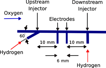
In this work, a nanosecond pulsed electric discharge was applied into the domain of a flat wall combustor configuration in accordance to the supersonic combustion experiment of Do et al. [51] following the proposed simplified numerical procedure. In this experiment, a custom-built test section with two fuel injectors and two electrodes embedded in a flat wall was located in an expansion tube in order to study the effect of a high-voltage nanosecond plasma discharge on the supersonic combustion of H2-O2 mixtures.
A schematic of the model representing the wall of the scramjet engine combustor used in the experiment is presented in Figure 2. In this configuration, a supersonic oxygen flow parallel to the wall enters the test section and encounters a rectangular aluminum plate with two fuel injectors flush with the model surface. The first injector, upstream, works as a pilot, injecting hydrogen to promote the generation of radicals once the plasma is applied. This injector is also tilted at an angle of $30^{\circ}$ or $60^{\circ}$ from the horizontal plane in order to promote the penetration of the fuel in the region near the wall and its further interaction with the electric discharge. The second injector, downstream, generates a transversal hydrogen jet that promotes the ignition via mixing. Two thoriated shape tungsten electrodes are inserted in the region between the two injectors. The electrodes generate a non-equilibrium electric discharge during 10 ns with a repetition rate of 50 kHz.
The penetration of the hydrogen jets into the main stream flow was specified using the jet to free-stream momentum ratio which is defined in Eq. (19).
$J_n=\sin (\theta) \cdot \frac{\left(\rho U^2\right)_{j e t}}{\left(\rho U^2\right)_{\infty}}$ (24)
Figure 2. Schematic of the flat wall model [53]
The non-equilibrium discharge was produced by repetitive 15 kV peak pulses, 10 ns pulse width and 50 kHz repetition rate. The voltage in the cathode and the anode was -7.5 kV and 7.5 kV peak respectively. An approximate nominal power of 10 W was consumed between the plasma pulses. That is each 20 µs. The energy of a pulse was about 0.2 mJ and the discharge volume was approximately 6 mm3. The reduced electric field of the pulsed discharge is estimated to be 300 Td.
In the experiment of Do et al. [51], eight cases with different flow conditions were tested corresponding to different pressure ratios of the sections of the expansion tube. Table 1 shows the run conditions for one of these eight cases. This was the case selected for validation in this work owing to its associated reported results showing OH PLIF images. For this case, the authors provided images displaying flames when two fuel injectors with and without applied plasma. The images are suitable to be benchmarked with the simulation results from this work showing how the supersonic combustion is enhanced by the application of the plasma.
Table 1. Selected run condition [51]
|
Property |
Oxygen |
|
Mach Number |
2.4±0.05 |
|
Stagnation Enthalpy (MJ/kg) |
2.4±0.08 |
|
Static Temperature (K) |
1300±50 |
|
Static Pressure (kPa) |
24±1 |
|
Test Time (μs) |
300±50 |
|
Flow Velocity (m/s) |
1690±30 |
3.1 Computational domain and flow conditions
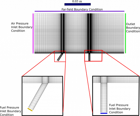
Figure 3 provides a schematic representation of the domain created to simulate the flat wall experiment. According to Do [49], the boundary layer thickness was about 0.1 mm. As a result, the vertical distance of the domain from the flat wall was set to 0.05 m. That is 500 times greater than the boundary layer thickness. A 33.7+k cells structured grid was built as is shown in Figure 3. Refinement was performed near the walls and within the region between the two injectors were shock waves and recirculation zones were expected. The regions where the fuel coming from the injectors enters the combustor were also refined since the area change from the injector to the combustor lead to recirculation zones and Mach disks. The lower distance in the y-direction was about 6×10⁻⁵ m near the flat wall of the combustor and the walls of the injectors, while in the x-direction was about 2×10⁻⁵ m in the regions where fuel encounters the free-stream flow and shock waves take place. These criteria were stablished, along with a time step value of 1.2×10⁻⁸ s, to achieve a courant number less than one with a mean stream flow velocity of 1960 m/s. The average aspect ratio and the average orthogonal quality of the mesh were of 6.32 and 0.99, respectively.
Figure 3. Computational mesh of the flat wall experiment
A convergence study was also performed to verify mesh independence from the number of cells elements. In addition to the 33.7 k cells mesh, 11.5 k, 21.7 k and 46.3 k cells meshes were built. Figure 4 shows the temperature profile along the horizontal distance of the simulation domain at a vertical distance of 0.01m from the wall. It can be observed that the temperature profiles of the 11.5 k, 21.7 k and 33.7 k cells meshes present differences from each other specially within the horizontal distance from 0.05 m to 0.06 m where shock waves and recirculation phenomena take place. This situation also is clear in the horizontal distance from 0.09 and 0.1 m Nonetheless, these differences are rather subtle between the 33.7 k and 46.3 k cells meshes. This last comparison indicates that the addition of more elements to the 33.7 k cells mesh do not lead to relevant changes in the numerical results.
Figure 4. Temperature profiles along the vertical distance of the flat wall combustor for different meshes
The boundary conditions for the simulation of the flat wall configuration of Do et al. [51] were established according to the run conditions in Table 1. Given that the flow information is provided in terms of momentum ratios, Jn, as shown in Eq. (24), where θ is the fuel injection angle, (U)jet is jet fuel velocity and (U)∞ is the free-stream velocity, pressure inlet boundary conditions were set as shown in Table 2. The momentum ratio for the upstream injector was 0.1 while the momentum ratio for the downstream injector was 2. No-slip condition, zero flux heat and zero diffusive flux species were assumed on the walls.
Table 2. Simulation flow conditions of the flat wall case
|
Property |
Oxidizer |
Upstream Injector |
Downstream Injector |
|
Mach Number |
2.40 |
0.75 |
1.00 |
|
Static Temperature (K) |
1300.00 |
295.00 |
295.00 |
|
Static Pressure (kPa) |
24000.00 |
26519.72 |
258375.97 |
|
H2 Mass Fraction |
0.00 |
1.00 |
1.00 |
|
O2 Mass Fraction |
1.00 |
0.00 |
0.00 |
3.2 Nanosecond pulsed discharge conditions
For the simulation, a nanosecond pulsed discharge configuration similar to that used [49, 51] was implemented in ZDplaskin. In this plasma discharge, a constant 300 Td reduced electric field with a 10 ns duration and 50 kHz frequency was assumed. This means that each 20 μs a plasma pulse is applied in the form of radical injection into the combustion domain. The initial electron density was set to 1018 m-3 according to the data provided by Do [49]. The time size step for the discharge simulation was set to 5×10⁻¹⁰ s.
4.1 OH radical analysis
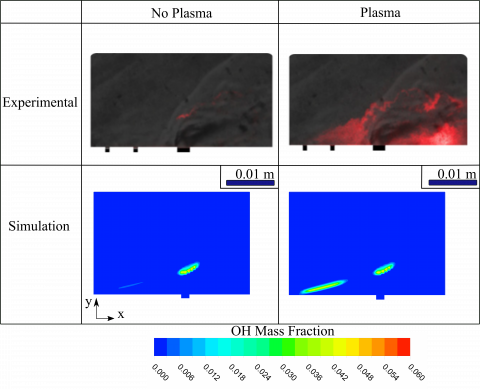
Figure 5 presents a comparison between experimental and simulation results regarding the presence of OH radicals inside the combustor. This, since the presence of OH radicals provide a good indication of ignition [49, 51]. While the experimental results are based on OH PLIF images overlapped with Schilieren images, the simulation results are displayed as contours of OH mass fraction. Results in this figure are 1 µs after a discharge pulse is applied. The upper of the side of the figure shows experimental images from [51] while the lower side displays contours obtained using the prosed simulation methodology.
It can be observed from the left side of the figure that, when no plasma is applied, a weak flame, detached from the wall, appears in both the experiments and the simulation. This phenomenon is attributed to the recirculation zone formed when fuel sonically enters into the combustor through the downstream injector blocking the main-stream flow and causing the oxygen flow and the fuel jets to gain more time to mix and ignite as explained by Do et al. [51]. In addition, temperature increments behind the bow shocks resulting from upstream and downstream injections promote combustion in this region via acceleration of the chemical kinetics.
Once plasma is applied, experimental results provide evidence of an enhanced flame. The right upper side of Figure 5 shows that on the left side of the downstream injector the flame seems to originate in the plasma application region due to the active radicals seeded and propagate into the main stream flow. It is observed that the flame follows the large structures formed by turbulence effects which foster the propagation of the flame and combustion.
From the right lower side of Figure 5, it can be noted that while the OH mass fraction contours retrieved from the simulation reveal a filamentary flame on the plasma application region, a deep propagation is not appreciated as in experimental results. This behavior is attributed to the lack of the large-scale coherent structures in the simulation as a result of the compressible Favre averaged turbulence model implemented. These large-scale coherent structures formed in this type of flow are important factors in enhancing mixing and promoting flame diffusion [21, 42].
Figure 5. Flat wall combustor experimental OH PLIF images [51] and simulation OH mass fraction contours at 1 µs after a plasma discharge comparison
The OH PLIF image on the right side of Figure 5 also shows a flame on the right side of the downstream injector which is not observed in the OH mass fraction contours. Ignition at this region is believed to be promoted by remnant air that was filling the test section before sonic hydrogen is injected [49]. In the simulation, however, all this region was occupied by hydrogen. This, due to the high momentum of the hydrogen flow when compared to the main stream oxygen current which prevents mixing.
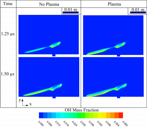
Figure 6 shows the simulation results for the contours of OH mass fraction that allow the visualization of flame enhancement due to the plasma application as time evolves. The left column depicts evidence that a flame is generated on the left side of the downstream injector without plasma assistance. In this case, the flame results from the upstream jet fuel and oxygen flow trapped in the recirculation region formed by the downstream injector and the temperature increased induced by the bow shock resulting from the fuel injection. On the other hand, the contours shown on the corresponding right column reveal that a higher concentration of OH appears in the same region at the same time when a discharge pulse is applied indicating the presence of a stronger flame and that combustion have been enhanced. Figure 6 reveals that this stronger plasma-ignited flame has been generated earlier than the auto-ignited flame. The upstream jet fuel serves as a pilot to generate radicals as a result of the electron impact plasma reactions with the mixture coming from the upstream region where the fuel was injected.
The set of results shown in Figures 5 and 6 indicate that the seeding of O and H radicals promotes a faster generation of radicals to trigger ignition but requiring less energy.
4.2 Temperature contours analysis
Figure 7 shows the contours of temperature retrieve from the simulation at 2 µs after a plasma discharge pulse. The upper side of the figure displays contours when no discharge is applied and the lower side shows contours when the plasma is applied. These contours allow to analyze the plasma effects on the flat wall flame from the temperature perspective. Even though experimental results do not provide information concerning temperature inside the combustor, the simulation results confirm the enhancement effect of the plasma on combustion.
Figure 6. Time evolution of OH mass fraction contours of the flat wall combustor simulation
Figure 7. Temperature contours of the flat wall at 2 µs after a plasma discharge. Upper side without plasma and lower side with plasma
In the absence of the plasma discharge a weak flame, represented by temperature increments in the contours originates on the left side of the downstream injector. In that region, the upstream hydrogen jet fuel and oxygen from the freestream flow mix and ignite due to recirculation and bow shocks temperature increments. In contrast, a stronger flame is generated when plasma seeded radicals react with the mixture leading to a faster energy release.
A comparison between experimental OH PLIF images and OH mass fraction contours revealed that a weak flame was formed when no plasma was applied in the flat wall combustor.
Despite the short time the air flow and the fuel jets have to mix and ignite due to the high speeds, ignition took place because of a recirculation region was created by sonic downstream injection of the hydrogen blocking the main stream flow. Experimental and numerical results revealed that the application of the plasma created a stronger flame.
Radicals added by the discharge shorten the ignition delay time by surpassing chain initiation reactions from the 18-steps mechanism selected for the model. This plasma effect compensates the high velocity convection on the mixture so more OH radicals are produced in less time in the region where plasma is applied. Even though this phenomenon is well reproduced by the proposed modeling approach, experimental results showed that the plasma-generated flame was broader than that in the numerical results and propagates following the large structures as a result of the turbulence. It is believed that the numerical flame differs from that in the experimental images because the turbulence model adopted does not capture the large structures, instead they are averaged. As a result, it is concluded that in order to have a more accurately reproduction of the experiment a Large Eddy Simulation (LES) is required. Nonetheless, it is quite clear that the proposed model is able to capture the main effects of the plasma inside the flat wall combustor at a lower computational burden than using LES.
This work was supported by the Universidad del Valle.
|
$A_r$ |
pre-exponential factor, m, kmol, s-1 |
|
$\beta_r$ |
temperature exponent |
|
$C_{m, r}$ |
molar concentration of species m in reaction r, kmol m-3 |
|
$c_{p, n}$ |
specific heat capacity at constant pressure of species n, J kg-1 K-1 |
|
$D_{T, n}$ |
thermal diffusion of species n, kg m-1 s-1 |
|
$D_n$ |
mass diffusion coefficient for species n in the mixture, m2 s-1 |
|
$D_{n, m}$ |
binary diffusion of species n in each species m, m2 s-1 |
|
$\tilde{e}$ |
Favre-averaged internal energy, J kg-1 |
|
$E$ |
total energy, J kg-1 |
|
$E_{a, r}$ |
activation energy for reaction r, J kmol-1 |
|
$\dot{\mathrm{G}}_k$ |
plasma species k generation/destruction term, m-3 s-1 |
|
$h$ |
enthalpy of the mixture, J kg-1 |
|
$h_n$ |
sensible enthalpy of species n, J kg-1 |
|
$\tilde{h}$ |
Favre-averaged enthalpy, J kg-1 |
|
$h^{\prime \prime}$ |
fluctuating-Favre enthalpy, J kg-1 |
|
$\mathrm{H}$ |
total enthalpy, J kg-1 |
|
$J_{n, j}$ |
diffusion flux of species n in direction j, kg m-2 s-1 |
|
$\mathrm{K}$ |
thermal conductivity of the mixture, W m-1 K-1 |
|
$\mathrm{K}_n$ |
thermal conductivity of the species n, Wm-1 K-1 |
|
$\mathrm{k}$ |
turbulence kinetic energy, m2 s-2 |
|
$k f_r$ |
forward rate constant for reaction r, kmole m-3 s-1, s-1, m3 mol-1 s-1 |
|
$K p_m$ |
plasma reaction rate coefficient, m-3 s-1 |
| $\mathcal{M}_n$ | symbol denoting species n |
|
$M_{W,n}$ |
molecular weight of species n, kg kmol-1 |
|
$N$ |
total number of chemical species in the system |
|
$N_R$ |
total number of reactions in the system |
|
$n_k$ |
number density of plasma species k, m-3 |
|
$\bar{P}$ |
Reynolds-averaged static pressure, kg m-1s-2 |
|
$P_{o p}$ |
operating pressure, kg m-1s-2 |
|
$Q_{k m}$ |
source terms for the species k corresponding to the contributions from different plasma reactions m, m-3 s-1 |
|
$R$ |
universal gas constant, J kmol-1 K-1 |
|
$R_n$ |
net rate of production of species n by chemical reactions, kg m-3 s-1 |
|
$\widehat{R_{n, r}}$ |
Arrhenius molar rate of creation/destruction of species n in reaction r, kmol m-3 s-1 |
|
$R p_m$ |
reaction rate of plasma species, m-3 s-1 |
|
$S_h$ |
volumetric heat source, J kg-1s-1 |
|
$S c_t$ |
turbulent Schmidt number |
|
t |
time, s |
| T | temperature, K |
| $\tilde{T}$ | Favre-averaged temperature, K |
|
$T_{r e f}$ |
reference temperature, K |
|
$\tilde{u}_l$ |
Favre-averaged velocity vector in i direction, m s-1 |
|
$u_i^{\prime \prime}$ |
fluctuating-Favre velocity vector in i direction, m s-1 |
|
$\tilde{u}_{\jmath}$ |
Favre-averaged velocity vector in j direction, m s-1 |
|
$u_j^{\prime \prime}$ |
fluctuating-Favre velocity vector in j direction, m s-1 |
|
$v_{n, r}^{\prime}$ |
stoichiometry coefficient for reactant n in reaction r |
|
$v_{n, r}^{\prime \prime}$ |
stoichiometry coefficient for product n in reaction r |
|
$x_i$ |
distance in i direction |
|
$x_j$ |
distance in j direction |
|
$X_n$ |
mole fraction of species n |
|
$X_m$ |
mole fraction of species m |
|
$Y_n$ |
local mass fraction of species n |
|
Greek symbols |
|
|
$\Gamma_k$ |
species k flux number, m-1 s-1 |
|
$\Gamma_{t b}$ |
net effect of third bodies on the reaction rate, mol m-3 |
|
$\gamma_{m, r}$ |
third body efficiency of the mth species in the r th reaction |
|
$\eta_{n, r}^{\prime}$ |
rate exponent for reactant species n in reaction r |
|
$\eta_{n, r}^{\prime \prime}$ |
rate exponent for product species n in reaction r |
|
$\mu_t$ |
turbulent dynamic viscosity, kg m-1 s-1 |
|
$\bar{\rho}$ |
Reynolds-averaged density, kg m-3 |
|
$\bar{\tau}$ |
averaged viscous shear stress tensor, kg m-1 s-2 |
|
$\psi_{n m}$ |
function of the properties of pure components of the mixture |
|
Subscripts |
|
|
$a$ |
activation |
|
$i$ |
direction i |
|
$j$ |
direction j |
|
mix |
mixture |
|
$m$ |
species m |
|
$n$ |
species n |
|
op |
operating |
|
$R$ |
total reactions |
|
r |
reaction rth |
|
ref |
reference |
|
$t b$ |
third body |
[1] Segal, C. (2009). The Scramjet Engine: Processes and Characteristics. Cambridge: Cambridge University Press. https://doi.org/10.1017/CBO9780511627019
[2] Jazra, T., Preller, D., Smart, M.K. (2013). Design of an airbreathing second stage for a rocket-scramjet-rocket launch vehicle. Journal of Spacecraft and Rockets, 50(2): 411-422. https://doi.org/10.2514/1.A32381
[3] Kanda, T., Kudo, K. (1997). Payload to low earth orbit by aerospace plane with scramjet engine. Journal of Propulsion and Power, 13(1): 164-166. https://doi.org/10.2514/2.7641
[4] Preller, D., Smart, M.K. (2017). Reusable launch of small satellites using scramjets. Journal of Spacecraft and Rockets, 54(6): 1317-1329. https://doi.org/10.2514/1.A33610
[5] Smart, M.K., Tetlow, M.R. (2009). Orbital delivery of small payloads using hypersonic airbreathing propulsion. Journal of Spacecraft and Rockets, 46(1): 117-125. https://doi.org/10.2514/1.38784
[6] Tetlow, M.R., Doolan, C.J. (2007). Comparison of hydrogen and hydrocarbon-fueled scramjet engines for orbital insertion. Journal of Spacecraft and Rockets, 44(2): 365-373. https://doi.org/10.2514/1.24739
[7] Fuhs, A. (1990). Future science and technology for military space. Space Programs and Technologies Conference, Huntsville, AL, USA. https://doi.org/10.2514/6.1990-3827
[8] Kamlet, M. (2017). NASA test flights to examine technology for improved supersonic flight efficiency on supersonic aircraft. NASA Armstrong Flight Research Center.
[9] Mitani, T. (1995). Ignition problems in scramjet testing. Combustion and Flame, 101(3): 347-359. https://doi.org/10.1016/0010-2180(94)00218-H
[10] Tian, Y. Yang, S., Xiao, B., Zhong, F., Le, J. (2019). Investigation of ignition characteristics in a kerosene fueled supersonic combustor. Acta Astronautica, 161: 425-429. https://doi.org/10.1016/j.actaastro.2019.03.024
[11] Scheuermann, T., Chun, J., Wolfersdorf J.V. (2008). Experimental investigations of scramjet combustor characteristics. 15th AIAA International Space Planes and Hypersonic Systems and Technologies Conference, Dayton, Ohio. https://doi.org/10.2514/6.2008-2552
[12] Gaston, M., Mudford, N., Houwing, F. (2012). A comparison of two hypermixing fuel injectors in a supersonic combustor. 36th AIAA Aerospace Sciences Meeting and Exhibit, American Institute of Aeronautics and Astronautics, Reno, NV, USA. https://doi.org/10.2514/6.1998-964
[13] Kodera, M., Sunami, T., Sheel, F. (2002). Numerical study on the supersonic mixing enhancement using streamwise vortices. AIAA/AAAF 11th International Space Planes and Hypersonic Systems and Technologies Conference, American Institute of Aeronautics and Astronautics, Orleans, France. https://doi.org/10.2514/6.2002-5117
[14] Ben-Yakar A., Hanson, R. (1999). Supersonic combustion of cross-flow jets and the influence of cavity flame-holders. 37th Aerospace Sciences Meeting and Exhibit. American Institute of Aeronautics and Astronautics, Reno, NV, USA. https://doi.org/10.2514/6.1999-484
[15] McMillin, B.K., Seitzman, J.M., Hanson, R.K. (1994). Comparison of NO and OH planar fluorescence temperature measurements in scramjet model flowfield. AIAA Journal, 32(10): 1945-1952. https://doi.org/10.2514/3.12237
[16] Correa S., Warren, R. (1989). Supersonic sudden-expansion flow with fluid injection - an experimental and computational study. 27th Aerospace Sciences Meeting, American Institute of Aeronautics and Astronautics, Reno, NV, USA. https://doi.org/10.2514/6.1989-389
[17] Dutton, J., Herrin, J., Molezzi, M., Mathur, T., Smith, K. (1995). Recent progress on high-speed separated base flows. 33rd Aerospace Sciences Meeting and Exhibit, American Institute of Aeronautics and Astronautics, Reno, NV, USA. https://doi.org/10.2514/6.1995-472
[18] Fletcher D., Mcdaniel, J. (1987). Quantitative measurement of transverse injector and free stream interaction in a nonreacting SCRAMJET combustor using laser-induced iodine fluorescence. 25th AIAA Aerospace Sciences Meeting, American Institute of Aeronautics and Astronautics, Reno, NV, USA. https://doi.org/10.2514/6.1987-87
[19] Sato, N., Imamura, A., Shiba, S., Takahashi, S., Tsue, M., Kono, M. (1999). Advanced mixing control in supersonic airstream with a wall-mounted cavity. Journal of Propulsion and Power, 15(2): 358-360. https://doi.org/10.2514/2.5433
[20] Yu, K.H., Schadow, K.C. (1994). Cavity-actuated supersonic mixing and combustion control. Combustion and Flame, 99(2): 295-301. https://doi.org/10.1016/0010-2180(94)90134-1
[21] Ben-Yakar A., Hanson, R.K. (2001) Cavity flame-holders for ignition and flame stabilization in scramjets: An overview. Journal of Propulsion and Power, 17(4): 869-877. https://doi.org/10.2514/2.5818
[22] Liu, Q., Baccarella, D., Lee, T., Hammack, S., Carter, C.D., Do, H. (2017). Influences of inlet geometry modification on scramjet flow and combustion dynamics. Journal of Propulsion and Power. 33(5): 1179-1186. https://doi.org/10.2514/1.B36434
[23] Heiser, W.H., Pratt, D., Daley, D., Mehta, U. (1994). Hypersonic airbreathing propulsion. AIAA Education Series, Washington, DC. https://doi.org/10.2514/4.470356
[24] Ombrello, T., Won, S.H., Ju, Y., Williams, S. (2010). Flame propagation enhancement by plasma excitation of oxygen. Part I: Effects of O3. Combustion and Flame, 157(10): 1906-1915. https://doi.org/10.1016/j.combustflame.2010.02.005
[25] Ombrello, T., Won, S.H., Ju, Y., Williams, S. (2010). Flame propagation enhancement by plasma excitation of oxygen. Part II: Effects of O2(a1Δg). Combustion and Flame, 157(10): 1916-1928. https://doi.org/10.1016/j.combustflame.2010.02.004
[26] Yin, Z., Adamovich, I.V., Lempert, W.R. (2013). OH radical and temperature measurements during ignition of H2-air mixtures excited by a repetitively pulsed nanosecond discharge. Proceedings of the Combustion Institute, 34(2): 3249-3258. https://doi.org/10.1016/j.proci.2012.07.015
[27] Sun, W., Uddi, M., Won, S.H., Ombrello, T., Carter, C., Ju, Y. (2012). Kinetic effects of non-equilibrium plasma-assisted methane oxidation on diffusion flame extinction limits. Combustion and Flame, 159(1): 221-229. https://doi.org/10.1016/j.combustflame.2011.07.008
[28] Smirnov, V.V., Stelmakh, O.M., Fabelinsky, V.I., Kozlov, D.N., Starik, A.M., Titova, N.S. (2008). On the influence of electronically excited oxygen molecules on combustion of hydrogen–oxygen mixture. Journal of Physics D: Applied Physics, 41(19): 192001. https://doi.org/10.1088/0022-3727/41/19/192001
[29] Mintusov, E., Serdyuchenko, A., Choi, I., Lempert, W.R., Adamovich, I.V. (2009). Mechanism of plasma assisted oxidation and ignition of ethylene – Air flows by a repetitively pulsed nanosecond discharge. Proceedings of the Combustion Institute, 32(2): 3181-3188. https://doi.org/10.1016/j.proci.2008.05.064
[30] Brumfield, B., Sun, W., Wang, Y., Ju, Y., Wysocki, G. (2014). Dual modulation faraday rotation spectroscopy of HO2 in a flow reactor. Optics letters, 39(7): 1783-1786. https://doi.org/10.1364/OL.39.001783
[31] Takita, K., Uemoto, T., Sato, T., Ju, Y., Masuya, G., Ohwaki, K. (2000). Ignition characteristics of plasma torch for hydrogen jet in an airstream. Journal of Propulsion and Power, 16(2): 227-233. https://doi.org/10.2514/2.5587
[32] Kimura, I., Aoki, H., Kato, M. (1981). The use of a plasma jet for flame stabilization and promotion of combustion in supersonic air flows. Combustion and Flame, 42: 297-305. https://doi.org/10.1016/0010-2180(81)90164-4
[33] Chen, D.C.C., Lawton, J., Weinberg, F.J. (1965). Augmenting flames with electric discharges. Symposium (International) on Combustion, 10(1): 743-754. https://doi.org/10.1016/S0082-0784(65)80218-1
[34] Haselfoot C.E., Kirkby, P.J. (2009). XLV. The electrical effects produced by the explosion of hydrogen and oxygen. The London, Edinburgh, and Dublin Philosophical Magazine and Journal of Science, 8(46): 471-481. https://doi.org/10.1080/14786440409463215
[35] Kobayashi, K., Mitani, T., Tomioka, S. (2004). Supersonic flow ignition by plasma torch and H2/O2 torch. Journal of Propulsion and Power, 20(2): 294-301. https://doi.org/10.2514/1.1760
[36] Bradley, D., Ibrahim, S.M.A. (1975). Electron temperatures in flame gases: Experiment and theory. Combustion and Flame, 24: 169-171. https://doi.org/10.1016/0010-2180(75)90144-3
[37] Jaggers H.C., Engel, A.V. (1971). The effect of electric fields on the burning velocity of various flames. Combustion and Flame, 16(3): 275-285. https://doi.org/10.1016/S0010-2180(71)80098-6
[38] Won, S.H., Ryu, S.K., Kim, Cha, M.S., Chung, S.H. (2008). Effect of electric fields on the propagation speed of tribrachial flames in coflow jets. Combustion and Flame, 152(4): 496-506. https://doi.org/10.1016/j.combustflame.2007.11.008
[39] Do, H., Cappelli, M., Mungal, G. (2010). Plasma assisted cavity flame ignition in supersonic flows. Combustion and Flame, 157(9): 1783-1794. https://doi.org/10.1016/j.combustflame.2010.03.009
[40] Voland, R., Rock, K. (2012). NASP concept demonstration engine and subscale parametric engine tests. International Aerospace Planes and Hypersonics Technologies, American Institute of Aeronautics and Astronautics, Chattanooga, TN, USA. https://doi.org/10.2514/6.1995-6055
[41] Breden, D., Raja, L. (2012). Simulations of nanosecond pulsed plasmas in supersonic flows for combustion applications. AIAA Journal, 50(3): 647-658. https://doi.org/10.2514/1.J051238
[42] Nagaraja, S. (2014). Multi-Scale modeling of nanosecond plasma assisted combustion. Ph. D. Thesis. School of Aerospace Engineering, Georgia Institute of Technology, Atlanta, GA, USA.
[43] Breden, D.P. (2013). Simulations of atmospheric pressure plasma discharges, Ph. D. Thesis. Department of Aerospace Engineering, The University of Texas at Austin, Austin, TX, USA.
[44] Ju, Y., Sun, W. (2015). Plasma assisted combustion: dynamics and chemistry. Progress in Energy and Combustion Science, 48: 21-83. https://doi.org/10.1016/j.pecs.2014.12.002
[45] Castela, M.L., Fiorina, B. Coussement, A., Gicquel, O., Darabiha, N., Laux, C. (2016). Modelling the impact of non-equilibrium discharges on reactive mixtures for simulations of plasma-assisted ignition in turbulent flows. Combustion and Flame, 166: 133-147. https://doi.org/10.1016/j.combustflame.2016.01.009
[46] Starikovskiy, A. (2015). Physics and chemistry of plasma-assisted combustion. Philosophical Transactions of the Royal Society a Mathematical, Physical and Engineering Sciences, 373(2048). https://doi.org/10.1098/rsta.2015.0074
[47] Bozhenkov, S.A., Starikovskaia, S.M., Starikovskii, A. Yu. (2003). Nanosecond gas discharge ignition of H2 − and CH4 − Containing mixtures. Combustion and Flame, 133(1-2): 133-146. https://doi.org/10.1016/S0010-2180(02)00564-3
[48] Stancu, G.D., Kaddouri, F., Lacoste, D.A., Laux, C.O. (2010). Atmospheric pressure plasma diagnostics by OES, CRDS and TALIF. Journal of Physics D: Applied Physics, 43(12): 124002. https://doi.org/10.1088/0022-3727/43/12/124002
[49] Do, H. (2009). Plasma-assisted combustion in a supersonic flow. Ph. D. Thesis. Department of Mechanical Engineering, Stanford University, Stanford, CA, USA.
[50] Guerra García, C.. (2011). High voltage repetitive pulsed nanosecond discharges as a selective source of reactive species. MSC thesis. Department of Aeronautics and Astronautics, Massachusetts Institute of Technology, Cambridge, MA, USA.
[51] Do, H., Im, S.K., Cappelli, M.A., Mungal, M.G. (2010). Plasma assisted flame ignition of supersonic flows over a flat wall. Combustion and Flame, 157(12): 2298-2305. https://doi.org/10.1016/j.combustflame.2010.07.006
[52] Pancheshnyi, S., Eismann, B., Hagelaar, G., Pitchford, L. (2008). ZDPlasKin: A new tool for plasmachemical simulations. Bulletin of the American Physical Society.
[53] Hagelaar, G.J.M., Pitchford, L.C. (2005). Solving the boltzmann equation to obtain electron transport coefficients and rate coefficients for fluid models. Plasma Sources Science and Technology, 14(4): 722-733. https://doi.org/10.1088/0963-0252/14/4/011
[54] Orszag, S. A., Yakhot, V., Flannery, W. S., Boysan, F. (1993). Renormalization group modeling and turbulence simulations. International Conference on Near-Wall Turbulent Flows, Tempe, Arizona, USA.
[55] Peters, N., Rogg, B. (1993). Reduced kinetic mechanisms for applications in combustion systems. Springer-Verlag, Berlin Heidelberg. https://doi.org/10.1007/978-3-540-47543-9
[56] ANSYS Inc. (2009). ANSYS FLUENT 12.0, Theory Guide.
[57] Yin, Z., Montello, A., Carter, C., Lempert, W., Adamovich, I. (2013). Measurements of temperature and hydroxyl radical generation/decay in lean fuel – air mixtures excited by a repetitively pulsed nanosecond discharg. Combustion and Flame, 160(9): 1594-1608. https://doi.org/10.1016/j.combustflame.2013.03.015
[58] Montello, A., Yin, Z., Burnette, D., Adamovich, I., Lempert, W. (2013). Picosecond CARS measurements of nitrogen vibrational loading and rotational/translational temperature in nonequilibrium discharges. Journal of Physics D: Applied Physics, 46(46): 464002. https://doi.org/10.1088/0022-3727/46/46/464002
[59] Starikovskaia, S.M., Kukaev, E.N., Kuksin, A. Yu., Nudnova, M.M., Starikovskii, A.Yu. (2004). Analysis of the spatial uniformity of the combustion of a gaseous mixture initiated by a nanosecond discharge. Combustion and Flame, 139(3): 177-187. https://doi.org/10.1016/j.combustflame.2004.07.005
[60] Kosarev, I.N., Aleksandrov, N.L., Kindysheva, S.V., Starikovskaia, S.M., Starikovskii, A. Yu. (2008) Kinetics of ignition of saturated hydrocarbons by nonequilibrium plasma: CH4-containing mixtures. Combustion and Flame, 154(3): 569-586. https://doi.org/10.1016/j.combustflame.2008.03.007
[61] Brown, P.N., Hindmarsh, A.C. (1989). Reduced storage matrix methods in stiff ODE systems. Applied Mathematics and Computation, 31: 40-91. https://doi.org/10.1016/0096-3003(89)90110-0
[62] Alves, L.L., Coche, P., Ridenti, M.A., Guerra, V. (2016). Electron scattering cross sections for the modelling of oxygen-containing plasmas. The European Physical Journal D, 70: 124. https://doi.org/10.1140/epjd/e2016-70102-1
[63] Yoon, J.S., Song, M.Y., Han, J.M., Hwang, S.H., Chang, W.S., Lee, B., Itikawa, Y. (2008). Cross sections for electron collisions with hydrogen molecules. Journal of Physical and Chemical Reference Data, 37: 913-931. https://doi.org/10.1063/1.2838023