Hamid Mekhtiche | Mounir Zirari | Giulio Lorenzini* | Hijaz Ahmad | Younes Menni | Houari Ameur | Redha Rebhi | Nima Khalilpoor | Abdelkader Korichi
© 2021 IIETA. This article is published by IIETA and is licensed under the CC BY 4.0 license (http://creativecommons.org/licenses/by/4.0/).
OPEN ACCESS
Thermal spraying involves surface treatment technologies in which a finely divided material is sprayed at high velocity and in a molten or semi-molten state onto the part to be covered. Their main application is the protection against wear, corrosion, and thermal effects. They also have functional properties (electrical, magnetic, etc.), which make them suitable for various industrial uses. The success and shelf life of plasma deposits depends to a large extent on the quality of the adhesion between the deposit and the substrate or between the lamella that constitute the deposit and which are generated by the impact of the powder particles crushing on the substrate. In this work, the spreading and solidification of an alumina particle on a substrate of the stainless-steel under the plasma projection conditions are investigated. The study is conducted by using the interaction fluid-structure (FSI) method in the ANSYS-code. This method is selected to determine the mechanical characteristics at the interface of the substrate particles during rolling. A focus is made on the increased role of the deformations developed during spreading at the surface interface of the substrate, the concentration of the stresses on the adhesion of the lamella, and consequently the coating quality.
alumina particle, finite element method, numerical simulation, interfacial dynamic behavior
The thermal spraying is part of the family of surface treatments. The principle is to produce the coating using a carrier gas is to melt the powder particles and project them onto substrates to produce the coating, the end to change some materials. A coating property achieved by thermal spraying is controlled and evaluated qualitatively by the extent of its porosity, hardness, surface roughness, oxide content, and the bonding strength. Several factors may affect the contacting process, such as the speed and size of the impact particles, as well as the characteristics of the particulate material. Some works have been published on the thermal spray coating by using both the experimental and numerical techniques [1-5]. Kamnis et al. [6] and Chandra et al. [7] modeled adequately the effect of fully molten droplets on a substrate and showed a better understanding of the deformation of particles and adhesion. At present, the physical phenomena that occur during the impact process and spreading the particles on the substrate may be modeled by numerical techniques, such as the VOF method (Volume of Fluid) [8, 9]. This method is based on fluid dynamics, and it is used in various applications to monitor the modification of the surface droplet during spreading. Zhang et al. [10] used this approach to inspect the high-speed effect and the solidification of a droplet of yttria-stabilized zirconia on an inclined substrate. They observed a critical angle of impact of about 44° for the splash of the drop. Zirari et al. [11] combined the finite element method with VOF and the equivalent specific heat technique for the control of solidification. They illustrated a significant influence of the state of fusion of the particle on the Lamella morphologies and adhesion to the substrate. Abdellah El-Hadj et al. [12] and by the same approach showed the importance of the temperature of the surrounding gas on the morphology of the lamella and the adhesion to the substrate. Pasandideh-Fard et al. [2] by the same method Eulerian on a 3D Cartesian grid showed the impact of a drop of metal on horizontal or inclined substrates. Their technique does not give a good precision since it does not properly describe the orientation of the free process the boundary conditions. This method depends heavily on the size of the cells and therefor does not allow a precision, as reported by Liu et al. [13] and Pasandideh-Fard [14]. In the Lagrangian method, the mesh forms with matter and it makes it possible to more accurately represent the free surface. But this method has difficulty in the case of large deformation due to significant distortions of the mesh elements. The first one model that addresses the spreading and solidification phenomena is those of Jones [15] and Madjeski [16]. They treated separately the spread of a lamella and solidification based on the assumption that the propagation speed of the solidification front in the strip is slower than the speed of impact of the particle. In this context, simulations of a large deformation should also be conducted [17]. Dykhuizen et al. [18] and Grujicic et al. [19] used a calculation code based on the mechanical/hydrodynamic coupling (CTH) to determine the significant deformation or violent shocks. Ls-Dyna and Abaqus have also been utilized to study the behavior of the particles impact by cold spray. Based on Johnson-Cook equation, Li and Gao [20] and Moridi et al. [21] combined analytical and numerical solutions to determine the critical speeds and erosion in the projection process cold. Cedelle [22] reported that this technique does not give a good precision, because the authors treated separately the spreading of as late and its solidification. The required time for the generation of a lamina is less than five microseconds for the times reading of the molten particle with a solidification, which may begin at the end of spreading and continue during 0.8-10 microseconds after impact.
The objective of this paper is to combine both methods Lagrangian and Eulerian in a fluid structure interaction technique, to follow the deformations of the particle with greater precision and without difficulty by the VOF numerical method of a hand, and secondly monitoring the development of stress and therefore the deformations in the substrate, for the purpose of checking the relationship between lamella formation and substrate deformation at the interface.
The majority of problems involving a fluid-structure interaction with a strong mating between the flow and the structure displacement are known by great displacements of the domain boundaries. The regions near the latter move naturally and are discretized with a Lagrangian approach. However, the conventional Eulerian approach with a fixed reference may be used for modeling the fluid areas that are located away from the moving borders.
The Navier-Stokes equations for incompressible fluid flows and constant viscosity are:
$\rho \alpha \frac{\partial u_{i}}{\partial t}+\rho u_{i} \alpha \frac{\partial u_{i}}{\partial x_{j}}=\frac{\partial \tau_{i j}}{\partial x_{j}}+b_{i}$ (1)
In the equation above, i, j=1, 2 are the spatial coordinates, t is the time variable, ρ is the density of the fluid, ui are the components of the velocity of the fluid, bi are the forces of external organism, and τij is the stress tensor. Eq. (1) is subject to the restriction of incompressibility, Cedelle [22]:
$\frac{\partial \propto \cdot u_{i}}{\partial x_{i}}=0$ (2)
and the stress tensor is given by:
$\tau_{i j=} \alpha \cdot p \cdot \delta_{i j}+\mu . \alpha\left(\frac{\partial u_{i}}{\partial x_{j}}+\frac{\partial u_{j}}{\partial x_{i}}\right)$ (3)
where, μ is the dynamic viscosity, p is the pressure, δij is the Kronecker coefficient, and α is the color variable. To indicate the absence or presence of the fluid, a fluid volume fraction is defined for each domain. The value “1” is set in the domain occupied by the metal and 0 for the remaining domain. The mean value in the element presents the function of the fluid volume occupied by the metal, Liu et al. [13]:
$\alpha=\left\{\begin{array}{c}1 \text { inside thefluid } \\ 0 \\ 0 \text { empty cell }\end{array}\right.$$<\alpha<1$ at the interface (4)
The element with a value of α between 0 and 1 is containing the free surface or the interface. To find (x, t) for all points of the domain it necessary to solve the transport equation:
$\frac{\partial \alpha}{\partial t}+V \nabla \alpha=\frac{d \alpha}{d t}$ with $\quad \alpha(x, 0)=\alpha_{0}(x)$ (5)
The Eqns. (1) to (5) are written for a fixed domain Ωf and for a time interval Δt.
In the substrate the stress is related to the deformations by:
$\{\sigma\}=[D]\left\{\varepsilon^{e l}\right\}$ (6)
{σ}: vector constraint=$\left[\sigma_{x} \sigma_{y} \sigma_{z} \sigma_{x y} \sigma_{y z} \sigma_{x z}\right]^{T}$
[D]: elasticity or matrix of elastic stiffness. For some anisotropic elements, defined by a complete matrix definition,
$\left\{\varepsilon^{e l}\right\}:\{\varepsilon\}-\left\{\varepsilon^{t h}\right\}$: elastic deformation vector
{ε}: total deformation vector =$\left[\varepsilon_{x} \varepsilon_{y} \varepsilon_{z} \varepsilon_{x y} \varepsilon_{y z} \varepsilon_{x z}\right]^{T}$
$\left\{\varepsilon^{t h}\right\}$: vector of thermal deformation. Eq. (6) may be also written as:
$\{\varepsilon\}=\left\{\varepsilon^{t h}\right\}+[D]^{-1}\{\sigma\}$ (7)
For the 3D case, the thermal deformation vector is:
$\left\{\varepsilon^{t h}\right\}=\Delta T\left\lfloor\alpha_{x}^{s e} \alpha_{y}^{s e} \alpha_{z}^{s e} 000\right\rfloor^{T}$ (8)
$\alpha_{x}^{s e}$: coefficient of thermal expansion in the x-direction. The flexibility matrix, $[D]^{-1}$ is written:
$[D]^{-1}=$$\left[\begin{array}{cccccc}1 / E_{x} & -v_{x y} / E_{x} & -v_{x z} / E_{x} & 0 & 0 & 0 \\ -v_{y x} / E_{y} & 1 / E_{y} & -v_{x z} / E_{x} & 0 & 0 & 0 \\ & & & & \\ -v_{z x} / E_{z} & -v_{z y} / E_{z} & 1 / E_{z} & 0 & 0 & 0 \\ 0 & 0 & 0 & 1 / G_{X Y} & 0 & 1 / G_{X Y} \\ 0 & 0 & 0 & 0 & 1 / G_{X Y} & 0 \\ 0 & 0 & 0 & 0 & 0 & 1 / G_{X Z}\end{array}\right]$ (9)
where, the typical terms are:
$E_{x}$: Young's modulus in the x direction.
$v_{x y}$: major Poisson's ratio.
$v_{y x}$: small Poisson's coefficient.
$G_{x y}$: shear modulus in the xy-plane. For the 2D case in addition, the matrix $[D]^{-1}$ is presumed symmetrical, so that:
$\frac{v_{y x}}{E_{y}}=\frac{v_{x y}}{E_{x}}$ (10)
The development of Eqns. (7) and (8) gives explicitly the three equations:
$\varepsilon_{x}=\alpha_{x} \Delta T+\frac{\sigma_{x}}{E_{x}}-\frac{v_{x y} \sigma_{y}}{E_{x}}$ (11)
$\varepsilon_{y}=\alpha_{y} \Delta T-\frac{v_{x y} \sigma_{x}}{E_{x}}+\frac{\sigma_{y}}{E_{y}}$ (12)
$\varepsilon_{x y}=\frac{\sigma_{x y}}{G_{x y}}$ (13)
where, the typical terms are:
$\varepsilon_{x}$: Direct deformation in the x direction,
$\sigma_{x}$: Direct constraint in the x direction,
$\varepsilon_{x y}$: Shear deformation in the xy-plane,@
$\sigma_{x y}$: Shear stress on the xy-plane. Eq. (6) may be developed by inverting first the Eq. (9), then combining this result with Eqns. (8) and (10) to explicitly give the three equations:
$\sigma_{x}=\frac{E_{x}}{h}\left(\varepsilon_{x}-\alpha_{x} \Delta T\right)+\frac{E_{y}}{h}\left(v_{x y}\right)\left(\varepsilon_{y}-\alpha_{y} \Delta T\right)$ (14)
$\sigma_{y}=\frac{E_{y}}{h}\left(\varepsilon_{y}-\alpha_{y} \Delta T\right)+\frac{E_{y}}{h}\left(v_{x y}\right)\left(\varepsilon_{x}-\alpha_{x} \Delta T\right)$ (15)
$\sigma_{x y}=G_{x y} \varepsilon_{x y}$ (16)
or:
$h=1-\left(v_{x y}\right)^{2} \frac{E_{y}}{E_{x}}$ (17)
The shear module (Gxy) is calculated as follows:
$G_{x y}=\frac{E_{x}}{2\left(1+v_{x y}\right)}$ (18)
The interaction between the fluid and structure at a mesh interface yields a pressure. In addition, the motion of structures generates a "fluid load".
The equations in matrix form that govern become:
$\left[M_{s}\right]\{\ddot{U}\}+\left[K_{s}\right]\{U\}=\left\{F_{s}\right\}+[R]\{P\}$ (19)
$\left[M_{f}\right]\{\ddot{P}\}+\left[K_{f}\right]\{P\}=\left\{F_{f}\right\}-\rho_{0}[R]^{T}\{\ddot{U}\}$ (20)
[R] is a coupling matrix that presents the effective area associated with each node on the fluid-structure interface (FSI). This matrix takes into consideration the normal vector direction that is defined for each pair of fluid faces, and the coincident structural element that comprises the interface surface. The quantities of structure and fluid charge that are generated at the fluid-structure interface are functions of unknown nodal degrees of freedom.
The table (Table 1) summarizes the properties of the materials used in the simulation.
Table 1. Properties of the materials under study
|
Properties |
Particle: Aluminum Alloy |
Substrat: Steel HT13 |
||
|
Density ρ (kg/m³) |
2570 |
7800 |
||
|
Viscosity μ (m²/s) |
T (℃) |
|
- |
|
|
0 700 |
105 1.0345×10⁻³ |
- |
||
|
Thermal conductivity k (W/m∙K) |
70 |
26 |
||
|
Liquid specific heat h (J/kg∙K) |
1000 |
- |
||
|
Thermal conductivity k (W/m∙K) |
T (℃) 400 500 630 |
144 147 70 |
T (℃) 300 400 500 600 700 |
15.0 16.5 18.0 19.5 20.9 |
|
Specific heat h (J/kg∙K) |
T (℃) 100 300 400 570 580 |
400 500 800 1050 1038 |
T (℃) 20 460 200 |
502 500 550 |
|
Young's Module E (GPas) |
|
T (℃) 300 400 500 600 700 |
200 193 185 177 169 |
|
|
Poisson coefficient |
|
T (℃) 300 400 500 600 700 |
0.267 0.246 0.251 0.271 0.295 |
|
|
Thermal expansion 10-6 (1/K) |
|
|
16 |
|
4.1 Spreading factor validation
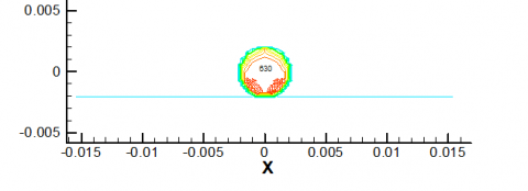
An example of validation proposed by Xue et al. [23] was considered here to illustrate the results of the contact/impact simulation using the FSI technique described above. The validation concerns a particle of aluminum alloy 380 with a diameter 3.92 mm and initial temperature 603℃ at a speed of 3m/s, impacting on a flat H13 tool steel substrate (of 12.5 mm by 3mm) at an initial temperature of 200℃ (Figure 1).
Figure 1. Geometric configuration and spreading conditions
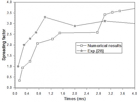
The variation of the spreading factor ($\zeta=d / D_{0}$) as a function of time during spreading and solidification on substrate is plotted alongside the experimental measurements in Figure 2. It seems that the same numerical and experimental results follow the same trend, where a good level of agreement is observed in terms of the droplets shape during the impact at all the stages of spreading.
Figure 2. Spreading factor
Moreover, the spatial presentation of the particle cooling during slat formation is illustrated in Figure 3. These results are dynamically similar to the propagation photographs of Xue et al. [23].
4.2 Influence of the impact dynamics on the lamella formation
Given the linear elastic material model described above, the FSI/VOF technique was used to illustrate the results of the particle/substrate interaction during the impact and lamella solidification. In this section, the influence of velocity variation at impact was examined for the same limit conditions of the problem.
(a) t=0.05 ms
(b) t=0.15 ms
(c) t=0.7 ms
(d) t=3 ms
(e) t=8 ms
Figure 3. Spatial presentation of the particle cooling during slat formation
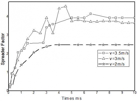
Figure 4 shows the variation over time of the impact factor for the three cases of velocity. For an impact velocity of 3m/s, the droplet reaches a spreading factor of maximum 4.5 at t=6.7ms and it decreases to an asymptotic value of approximately 3.72.
Figure 4. Spreading factor for the three cases
(a) u=2 m/s
(b) u=3 m/s
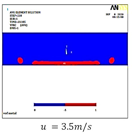
(c) u=3.5 m/s
Figure 5. The shape of lamella for the three cases studied
The effect of the dynamic variation of the impact on the spreading factor was studied here. The variation of the propagation factor vs. time and for several impact velocity values shows that the maximum values of spreading factor stabilize around 2.4 and 4 when u=2m/s and 3.5m/s, respectively.
For a good interpretation of these results, the three shapes of lamellae that result from the impact of the three cases studied are illustrated in Figure 5. As observed, the thickness of lamella decreases for u=3.5m/s compared to the reference case (u=3 m/s), resulting thus in an improvement in the rate of solidification and in the absence of recoil phenomena. Unfortunately, the lamella breaks out partially for this case, resulting thus in the formation of air pockets during the stacking of layers. In the case where the speed is lower than the reference speed (u=3 m/s), the particle does not spread and the deformation kinetic energy is lower than the viscous forces.
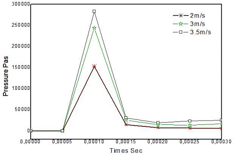
Figure 6 presents the pressure distributions under the droplet impact for the three cases studied. The impact velocity is found to be proportional to the impact pressure, which allows a more or less important contact in cases where the velocity is greater than 2m/s and the pressure generated is (~250 kPa). The impact velocity has a direct influence on the spreading time of the drop and on the maximum diameter reached by the lamella.
Figure 6. Pressure of the impact for the cases studied
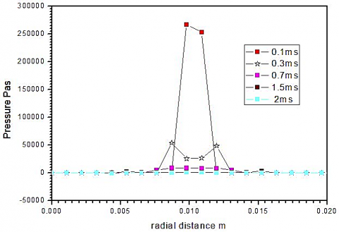
Figure 7 shows the pressure distribution at the spread interface and for various periods. For the two cases of speed (u=3m/s and 3.5m/s) and at the moment of impact, the pressure reaches a peak of 200 kPas after a time of about 0.1ms. This pressure acts a small radiating contact area of the order of 2mm.
(a) u=3.5 m/s
(b) u=3 m/s
Figure 7. Sequential impact pressure
4.3 Deformation and stress concentration on substrate
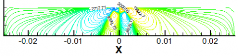
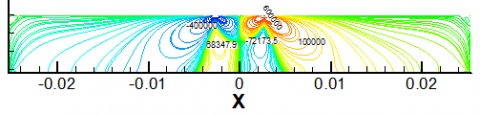
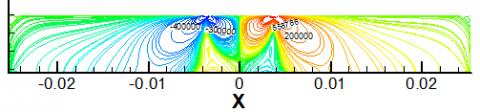
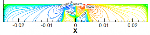
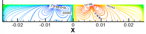
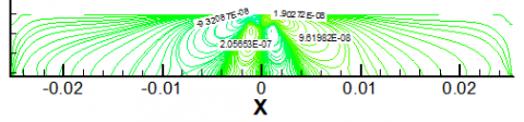
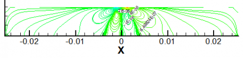
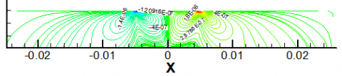
The stress concentration on the substrate and the related deformations are inspected here to give a mechanical explanation of the particle/substrate interaction. In Figure 8, the temporal distribution of the stresses (xy stress) is presented in the xy plane of substrate and for different values of velocity.
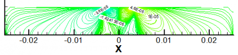
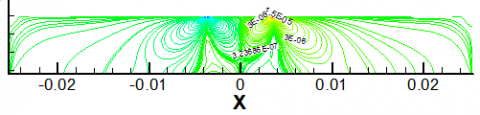
It should be noted that the particle deformation after the impact against the substrate and during spreading yields a frictional shear of the thin layers adjacent to the surface at the level of the surrounding zone. The interaction of these layers near the surface generates the residual tensile stress near the surface in the vicinity (Figures 8 and 9). The level of stress is high when the velocity is significant and it propagates radially on the contact interface and almost with the same intensity. The spatial presentation of the stresses developed in the substrate also shows a symmetry of intensity and traveling with the edges of the particle. This intensity is continually absorbed inside the substrate gradually. For the third case of velocity (u=3.5 m/s), the substrate thickness did not absorb the increase of the stress transversely, where a considerable radial stress development is observed. It can be said that the radial propagation of the stresses causes more radial deformations, which yields a partial splattering of the lamella.
(a) At t=0.1 ms for u=2, 3 and 3.5 m/s, respectively
(b) At t=0.7 ms for u=2, 3 and 3.5 m/s, respectively
(c) At t=3 ms for u=2, 3 and 3.5 m/s, respectively
Figure 8. XY stress spatial representation for the three case studies
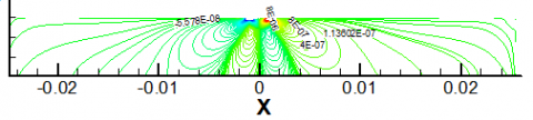
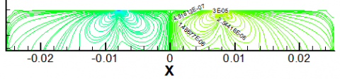
(a) At t=0.1 ms for u=2, 3 and 3.5 m/s, respectively
(b) At t=0.7 ms for u=2, 3 and 3.5 m/s, respectively
(c) At t=3 ms for u=2, 3 and 3.5 m/s, respectively
Figure 9. Spatial presentation of the XY strain for the three cases studies
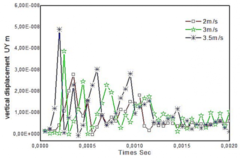
Figure 10. Vertical displacement of the impact point over time
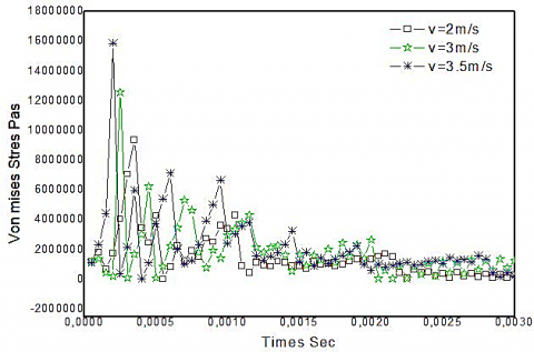
Figures 10 and 11 show, respectively, the history of the vertical displacement and the corresponding Von misses stress on the impact point of the substrate from impact to the final cooling. These results were obtained by using the thermally coupled model. It seems that the impact induces max stresses presented by peaks and generates displacements of the vertical deformation in the substrate. These stresses are relaxed during spreading, as illustrated by the oscillation with peaks decreasing until equilibrium.
Figure 11. Von misses stress of the impact point over times
In the case of u=3.5 m/s and t=1.5 ms, the stresses are relatively significant and provoke tension stress on the particle, which justifies the partial splashing of the latter to find a new state of equilibrium with the establishment of a new mechanical equilibrium.
This study was conducted aiming to provide further details on the dynamic and thermal phenomena that appear on the macro metric scale. The mechanical and thermal behavior of the spreading of an alumina particle on steel substrate by were numerically inspected by using the FSI model that is based on the finite element discretization method. Three cases of impact velocity were considered. The validation of our predictions against the experimental data revealed a good agreement for the different cases considered. The model used thus showed that an impact velocity lower than the reference speed does not allow the formation of a lamella, whereas for a higher speed the lamella splashes partially or totally proportional to the speed of impact.
The distribution of the stress and strain fields in the substrate and the interface were also examined. It was observed that the concentration of relatively high stresses at the interface for significant speeds could cause deformations that propagate along the interface, creating thus a splashing and critical size of adhesion defects.
[1] Pasandideh-Fard, M., Bhola, R., Chandra, S., Mostaghimi, J. (1998). Deposition of tin droplets on a steel plate: Simulations and experiments. International Journal of Heat and Mass Transfer, 41(19): 2929-2945. https://doi.org/10.1016/S0017-9310(98)00023-4
[2] Pasandideh-Fard, M., Chandra, S., Mostaghimi, J. (2002). A three-dimensional model of droplet impact and solidification. International Journal of Heat and Mass Transfer, 45(11): 2229-2242. https://doi.org/10.1016/S0017-9310(01)00336-2
[3] Kamnis, S., Gu, S., Vardavoulias, M. (2011). Numerical study to examine the effect of porosity on in-flight particle dynamics. Journal of Thermal Spray Technology, 20(3): 630-637. https://doi.org/10.1007/s11666-010-9606-9
[4] Gunghas, A., Kumar, R., Deswal, S., Kalkal, K.K. (2019). Influence of rotation and magnetic fields on a functionally graded thermoelastic solid subjected to a mechanical load. Journal of Mathematics. https://doi.org/10.1155/2019/1016981
[5] Higazy, M., Aggarwal, S., Hamed, Y.S. (2020). Determination of number of infected cells and concentration of viral particles in plasma during HIV-1 infections using Shehu transformation. Journal of Mathematics. https://doi.org/10.1155/2020/6624794
[6] Kamnis, S., Gu, S. (2005). Numerical modelling of droplet impingement. Journal of Physics D: Applied Physics, 38(19): 3664-3673. https://doi.org/10.1088/0022-3727/38/19/015
[7] Chandra, S., Fauchais, P. (2009). Formation of solid splats during thermal spray deposition. Journal of Thermal Spray Technology, 18(2): 148-180. https://doi.org/10.1007/s11666-009-9294-5
[8] Raessi, M., Mostaghimi, J. (2005). Three-dimensional modeling of density variation due to phase change in complex free surface flows. Numerical Heat Transfer B, 47(6): 507-531. https://doi.org/10.1080/10407790590928964
[9] Zhao, Z., Poulikakos, D., Fukai, J. (1996). Heat transfer and fluid dynamics during the collision of a liquid droplet on a substrate - I. Modeling. International Journal of Heat and Mass Transfer, 39(13): 2771-2789. https://doi.org/10.1016/0017-9310(95)00305-3
[10] Zhang, M.Y., Zhang, H., Zheng, L.L. (2008). Simulation of droplet spreading, splashing and solidification using smoothed particle hydrodynamics method. International Journal of Heat and Mass Transfer, 51(13-14): 3410-3419. https://doi.org/10.1016/j.ijheatmasstransfer.2007.11.009
[11] Zirari, M., Abdellah El-Hadj, A., Bacha, N. (2010). Numerical analysis of partially molten splat during thermal spray process using the finite element method. Applied Surface Science, 256(11): 3581-3585. https://doi.org/10.1016/j.apsusc.2009.12.158
[12] Abdellah, El-Hadj, A., Zirari, M., Bacha, N. (2010). Numerical analysis of the effect of the gas temperature on splat formation during thermal spray process. Applied Surface Science, 257(5): 1643-1648. https://doi.org/10.1016/j.apsusc.2010.08.115
[13] Liu, H., Lavernia, E., Rangel, R. (1993). Numerical simulation of impingement of molten Ti, Ni and W droplets on a flat substrate. Journal of Thermal Spray Technology, 2(4): 369-378. https://doi.org/10.1007/BF02645867
[14] Pasandideh-Fard, M., Mostaghimi, J. (1996). Droplet impact and solidification in a thermal spray process: droplet-substrate interaction. Thermal Spray 1996: Practical Solution for Engineering Problems, 637-646.
[15] Jones, H. (1971). Cooling, freezing and substrate impact of droplets formed by rotary atomization. Journal of Physics D: Applied Physics, 4(11): 1657-1660. https://doi.org/10.1088/0022-3727/4/11/206
[16] Madejski, J. (1976). Solidification of droplets on a cold surface. International Journal of Heat and Mass Transfer, 19(9): 1009-1013. https://doi.org/10.1016/0017-9310(76)90183-6
[17] Aalami-aleagha, M.E., Feli, S., Eivani, A.R. (2010). FEM simulation of splatting of a molten metal droplet in thermal spray coating. Computational Materials Science, 48(1): 65-70. https://doi.org/10.1016/j.commatsci.2009.12.002
[18] Dykhuizen, R.C., Smith, M.F., Gilmore, D.L., Neiser, R.A., Jiang, X., Sampath, S. (1999). Impact of high velocity cold spray particle. Journal of Thermal Spray Technology, 8(4): 559-564. https://doi.org/10.1361/105996399770350250
[19] Grujicic, M., Saylor, J.R., Beasley, D.E., De Rosset, W.S., Helfritch, D. (2003). Computational analysis of the interfacial bonding between feed-powder particles and the substrate in the cold-gas dynamic-spray process. Applied Surface Science, 219(3-4): 211-227. https://doi.org/10.1016/S0169-4332(03)00643-3
[20] Li, W.Y., Gao, W. (2009). Some aspects on 3D numerical modeling of high velocity impact of particles in cold spraying by explicit finite element analysis. Applied Surface Science, 255(18): 7878-7892. https://doi.org/10.1016/j.apsusc.2009.04.135
[21] Moridi, A., Hassani-Gangaraj, S.M., Guagliano, M. (2013). A hybrid approach to determine critical and erosion velocities in the cold spray process. Applied Surface Science, 273: 617-624. https://doi.org/10.1016/j.apsusc.2013.02.089
[22] Cedelle, J. (2005). Etude de la formation de lamelles résultant de l’impact de gouttes millimétriques et micrométriques: application à la réalisation d’un dépôt par projection plasma. Ph.D. thesis, Université de Limoges.
[23] Xue, M., Heichal, Y., Chandra, S., Mostaghimi, J. (2007). Modeling the impact of molten droplet on a solid surface using variable interfacial thermal contact resistance. Journal of Materials Science, 42(1): 9-18. https://doi.org/10.1007/s10853-006-1129-x