Nasim Ullah
© 2020 IIETA. This article is published by IIETA and is licensed under the CC BY 4.0 license (http://creativecommons.org/licenses/by/4.0/).
OPEN ACCESS
Standalone DC micro-grid requires highly efficient power converters with high performance robust controllers. This research work deals with the hardware implementation of a load side buck converter and its control system integrated in a DC micro-grid system. This paper presents a novel fractional order sliding mode control (FSMC) method for voltage regulation of a buck converter feeding a constant power load. FSMC controller is derived based on the average state space model of the buck converter and its stability is verified using Lyapunov theorem. Finally, the FSMC controller is implemented using Arduino mega 2560 processor and the obtained results are compared with classical sliding mode control (SMC), proportional, integral, derivative (PID) control and fractional order PID control system (FOPID under constant and variable resistive loading.
DC-DC converters, DC nano grid, fractional order sliding mode controllers, fractional calculus, variable resistive loading
Direct current (DC) micro-grid is an emerging research topic in recent times. The advantages of the DC grids over alternative current (AC) grids include better reliability, power efficiency and simpler architecture [1]. Due to the recent advancements in power semiconductor technology and enhanced computational power of processors the DC distribution is becoming the most feasible solution for both the industrial and residential loads. AC grids are complex, and many vital parameters are required to be taken care for its proper operation. These include the power factor, reactive power compensations, frequency and phases. In comparison to the AC grids, DC distribution does not require the control of the above all parameters [2-4]. A 10kwatts experimental prototype for a DC micro-grid is presented in reference [5].
Later, several other researchers extended the idea and developed several other applications of the DC micro-grids such as power backup source for telecommunication systems [6], distributed generation [7], data centers [8], and consumer loads [9]. Based on the voltage levels, reliability, stability and standardization of the components, several topologies have been proposed for DC microgrids such as single bus topology [10, 11], multi bus topology [12, 13] and reconfigurable topology [14].
The stability study for the DC micro-grids under the constant power loading is another important research area and in the recent times many researchers are focused on the stability issues of the DC micro-grid integrated converters. The stability issues of micro-grid integrated DC-DC converters have been reported by Cupelli et al. [15], AL-Nussairi et al. [16] and Asghar et al. [17]. The stability issues are generally addressed using closed loop techniques and the details have been discussed by Asghar et al. [17]. Apart from the stability issues, feedback control system needs to be carefully selected for optimal performance of DC micro-grids. DC micro-grids are interfaced through controllable power converters both at the source and load sides with a common DC link bus, thus voltage regulation is the control priority. To regulate DC link voltage for a micro-grid, the most widely utilized method is the droop control, which works on the cooperative sharing of the power or current among several converters [18, 19]. Droop control emulates a virtual resistance (VR) control loop along with the voltage loop [20, 21]. There are several limitations of the droop control method such as the load dependency in the voltage equation. The load dependency over the voltage causes a low efficiency of the current sharing algorithm. To solve this issue, secondary and tertiary controllers are proposed in the literature [3].
The droop control method limits the capability of the closed loop system in providing the desired coordinated performance of several components with different characteristics. Thus decentralized, centralized or distributed supervisory controllers are required to establish a specific mode such as droop control or maximum power point tracking (MPPT) [22, 23] or energy storage mode [24] should be adopted. Apart from the voltage and current regulation problem, stability of the DC micro-grid needs to be ensured over a wide range of operation. Points of load converters are tightly regulated, and it poses a challenge from the point of view of a negative impedance characteristic within the bandwidth of the applied control loops [25]. The negative impedance characteristic reduces the overall damping of the closed loop and it may lead to the instability of the whole system.
Apart from droop control schemes, several linear and nonlinear methods have been proposed for the control problem of DC micro-grids in the literature.
To design a linear control system, the model linearization technique is used for buck converter system [26]. Apart from its simple practical implementation, linear control methods lack the ability of handling uncertainties and parameter variation. Moreover, the converter operating point depends on the small signal model parameters [27]. Due to the variation of the system parameters and large signal transient changes in the load, the above linear controllers are not able to ensure system stability [28]. Similarly proportional, integral and derivative (PID) controller fails to perform optimally because of the non-linear dynamics of the power converters; and especially for point of load converters [29].
Nonlinear controllers are capable for compensating the disturbances and uncertainties in the parameter with fast transient response. Some nonlinear control methods have been discussed in the literature such as fuzzy sliding mode control [30, 31], robust sliding mode control [32, 33], optimal control [34], feedback linearization [35], adaptive control [36, 37] and extended state observer based control [38, 39] for the DC-DC converter. All the cited methods above are integer order and there are few research articles reported on the non-integer (fractional order) control of DC microgrid integrated power converters.
Recently, fractional order control (FOC) has emerged as a new choice to control both linear and nonlinear systems. It utilizes the attributes of fractional integrals and derivatives in the control schemes. A brief theoretical analysis of fractional operators has been discussed by Delghavi et al. [40] and Matignon [41], whereas the tuning of FOC schemes has been explained by Aghababa [42] and Li and Deng [43] for achieving optimal controls performance.
Linear FOC control schemes have been proposed for buck converter system by Calderon et al. [44] and Monje et al. [45]. In comparison to integer order controllers, fractional order methods offer superior performance due to an extra degree of freedom. However, the FOC control schemes utilize high computational resources when implemented over processors. This statement is verified in an experimental study published recently [46]. Apart from linear FOC control schemes, several nonlinear non integer methods have also been reported in the literature. Stability of fractional order nonlinear systems is discussed by Li et al. [47] while a generalized approach for tuning and auto tuning of FOC controllers is proposed by Monje et al. [48]. By choosing suitable non integer sliding surfaces, the FOC controllers consume less memory and less power over processors [46].
Based on the above literature survey, this article formulates a novel fractional order sliding mode control (FSMC) for a point of load buck converter. The proposed controller is derived based on fractional order sliding manifold. The stability of the proposed control scheme is proved using Lyapunov theorem. The proposed control scheme is implemented using Matlab/Simulink and Arduino mega 2560 hardware. Finally, the comparison of the proposed FOSMC controller is done with classical SMC, PID and fractional order PID controllers (FOPID) controllers.
Fractional order calculus finds several interesting applications in applied mathematics branch especially where the integrals and differentiators are applied. Fractional order calculus is applied to convert the integer integrators and differentiators in to fractional ones of any complex or real order. Fractional order operator is symbolized by $a D_{t}^{\alpha}$ and it can be defined as follows [45]:
${ }_{a} D_{t}^{\alpha} \cong D^{\alpha}=\left\{\begin{array}{cl}\frac{d^{\alpha}}{d t^{\alpha}} & , R(\alpha)>0 \\ 1 & , R(\alpha)=0 \\ \int_{a}^{t}(d \tau)^{-\alpha}, & R(\alpha)<0\end{array}\right.$ (1)
Here α and t represents the operating limts, α is the order of fractional operator and R is the real part of alpha. The fractional differentiator and integrator introduced by Riemann Liouville definition is given as follows [45]:
$_{a} D_{t}^{\alpha} f(t)=\frac{d^{\alpha}}{d t^{\alpha}} f(t)$
$=\frac{1}{\Gamma(m-\alpha) d t^{m}} \int_{\alpha}^{t} \frac{f(\tau)}{(t-\tau)^{\alpha-m+1}} d \tau$ (2)
${ }_{a} D_{t}^{-\alpha} f(t)=I^{\alpha} f(t)=\frac{1}{\Gamma(\alpha)} \int_{\alpha}^{t} \frac{f(\tau)}{(t-\tau)^{1-\alpha}} d \tau$ (3)
In Eq. (3), Γ(.) represents the Euler’s gamma function and can be defined as follows:
$\Gamma(x)=\int_{0}^{\infty} e^{-t} t^{(x-1)} d t, x>0$ (4)
The fractional order derivative and integrator defined by Grunwald Letnikov method is given as:
$a^{G L} D_{t}^{\alpha} f(t)=$
$\lim _{h \rightarrow 0} \frac{1}{h^{\alpha}} \sum_{j=0}^{[(t-\alpha) / h]}(-1)^{j}\left(\begin{array}{l}\alpha \\ j\end{array}\right) f(t-j h)$ (5)
Block diagram of a DC micro-grid is given in Figure 1. The micro-grid consists of sources such as photo-voltaic (PV), fuel cell and AC grid. Each source is integrated to the DC link via source side converters. Similarly, loads are driven using load side converters. Moreover, the battery storage system is integrated to the DC link via a dual active bridge. DC link is used to store and supply instantaneous energy from the source and to the loads respectively. As shown in the block diagram, the scope of this work to test the proposed controllers for a load side converter that drives a variable resistive load.
To derive the fractional order robust control system, it is necessary to derive an average state model of the system as a first step. By following the standard concepts of the switched mode power converters, the operation of the buck converter is divided in to two states. Figure 2 shows circuit diagram of a buck converter.
Figure 1. DC micro-grid block diagram
Figure 2. Circuit diagram of buck converter
Overall there are two states of the Mosfet switch. It can either be opened or in closed state. Thus, based on the two switching states, two equations are derived that represent the dynamics of the system. Consider the following two cases:
State 1: When the Mosfet switch is closed
When the Mosfet conducts then the converter dynamics are expressed as follows:
$V_{i}=L \dot{I}_{L}+V_{0}$ (6)
$C \dot{V}_{0}=I_{L}-\frac{V_{0}}{R_{L}}$ (7)
State 2: When the Mosfet switch is open
When the Mosfet switch is open so no curent flows from voltage source, then the stored energy in the inductor coil is released through the freewheeling diode and the system dynamics are represented as follows:
$L \dot{I}_{L}=-V_{0}$ (8)
$C \dot{V}_{0}=I_{L}-\frac{V_{0}}{R_{L}}$ (9)
Here Vi represents the input voltage, V0 is the output voltage, IL is the inductor current, L represents the inductance, C represents the capacitance and RL is the load.
The average state space model of the buck converter is derived as following [21]:
$L \dot{I}_{L}=u V_{i}-V_{0}$ (10)
$C \dot{V}_{0}=I_{L}-\frac{V_{0}}{R_{L}}$ (11)
Taking into account the parametric uncertainties of the system, the system of Eq. (11) is further elaborated as follows:
$\frac{d}{d t} I_{L}=\frac{u V_{i}}{L}-\frac{V_{0}}{L}+d_{i}$
$\frac{d}{d t} V_{0}=\frac{I_{L}}{C}-\frac{V_{0}}{R_{L} C}+d_{v}$ (12)
The terms di and dv represent parametric and load uncertainties in the power stage parameters represented as follows:
$d_{v}=\frac{u V_{i}}{\Delta L}-\frac{V_{o}}{\Delta L}$
$d_{i}=\frac{I_{L}}{\Delta C}-\frac{V_{o}}{\Delta R_{L} \Delta C}$ (13)
The uncertainties in power stage parameters L/C and load perturbations can occur due various reason such as: (a) aging effect of the converter due to its prolonged operating time, (b) thermal effects; as the parameters are directly effected by the change in temperature (c) load variations $\Delta R_{L}$.
In this section FSMC law is derived using system of Eq. (12). A fractional order sliding surface SV is defined as follows:
$S_{V}=c_{1} D^{-\alpha}\left(V_{r}-V_{0}\right)+c_{2} \int\left(\dot{V}_{r}-\dot{V}_{0}\right)$ (14)
In Eq. (14), c1, c2 represents the sliding surface constants, Vr shows the reference voltage command and V0 is the output voltage. By taking the fractional order derivative Dα on both sides of Eq. (14), one obtains the following relation [42]:
$D^{\alpha} S_{V}=c_{1}\left(e_{V}\right)+c_{2} D^{\alpha-1}\left(\dot{e}_{V}\right)$ (15)
Here eV=Vr-V0, while its first derivative is expressed as follows: $\dot{e}_{V}=\dot{V}_{r}-\dot{V}_{0}$. Expanding Eq. (15) in terms of the capacitor voltage dynamics, the resultant expression is given by Eq. (16).
$D^{\alpha} S_{V}=c_{1}\left(e_{V}\right)+c_{2} D^{\alpha-1}\left\{\dot{V}_{r}-\left(\frac{I_{L}}{C}-\frac{V_{0}}{R_{L} C}+d_{V}\right)\right\}$ (16)
Using Eq. (16), the current reference IL-ref can be generated as follows:
$I_{L-r e f}=\frac{C}{c_{2}}\left\{c_{2} \frac{V_{0}}{R_{L} C}+\dot{V}_{r}+D^{1-\alpha}\left(K_{1} S_{V}+c_{1} e_{V}\right)\right\}$ (17)
A current sliding surface SI is defined as follows:
$S_{I}=c_{3} D^{-\alpha}\left(I_{L-r e f}-I_{L}\right)+c_{4} \int\left(\dot{I}_{L-r e f}-\dot{I}_{L}\right)$ (18)
In Eq. (18), c3, c4 are the current sliding surface constants, and IL is the inductor current. By taking the fractional order derivative Dα on both sides of Eq. (18), one obtains the following relation:
$D^{\alpha} S_{I}=c_{3}\left(e_{I}\right)+c_{4} D^{\alpha-1}\left(\dot{e}_{I}\right)$ (19)
Here eI=IL-ref -IL is the current error, while its first derivative is expressed as follows: $\dot{e}_{I}=\dot{I}_{L-r e f}-\dot{I}_{L}$.
By including the dynamics of inductor current, Eq. (19) is further expanded as follows:
$D^{\alpha} S_{I}=c_{3}\left(e_{I}\right)+c_{4} D^{\alpha-1}\left\{\dot{I}_{L-r e f}-\left(\frac{u V_{i}}{L}-\frac{V_{0}}{L}+d_{i}\right)\right\}$ (20)
The current control law is derived as follows:
$\left\{\begin{array}{l}
u=u_{e q}+u_{s} \\
u_{e q}=\frac{L}{V_{i}}\left\{D^{1-\alpha}\left(\frac{c_{3}}{c_{4}} e_{I}\right)+\frac{V_{0}}{L}+\dot{I}_{L-r e f}\right\} \\
u_{s}=\frac{L}{V_{i}}\left\{D^{1-\alpha}\left(\frac{K_{2}}{c_{4}} \operatorname{sgn}\left(S_{I}\right)\right)\right\}
\end{array}\right.$ (21)
In Eq. (21), K1 and K2 represent the control system constants.
4.1 Stability proof
A Lyapunov theorem given by Aghababa [42] is utilized to prove the closed loop stability with the prooposed control scheme. The overall system’s stability will be proved in two steps. In the first step voltage loop is analyzed followed by the current loop. The following theorem is utilized to prove the stability.
Theorem 1: The proposed FSMC controller derived in Eq. (17) and (21) for the system given in Eq. (12) is stable if the following inequality holds true [18]:
$\left|\sum_{j=1}^{\infty} \frac{\Gamma(1+\alpha)}{\Gamma(1-j+\alpha) \Gamma(1+j)} D^{j} S_{V} D^{\alpha-j} S_{V}\right| \leq \Omega_{1}\left(S_{V}\right)$ (22)
Here SV, represents the voltage sliding surface and Ω1(.) is a positive constant.
4.2 Proof for voltage loop
To prove the stability of the voltage loop, the Lyapunov candidate function is defined as follows:
$V_{V}=\frac{1}{2} S_{V}^{2}$ (23)
Applying Dα to Eq. (23) yields the following expression [42]:
$D^{\alpha} V_{V}=S_{V} D^{\alpha} S_{V}+\left|\sum_{j=1}^{\infty} \frac{\Gamma(1+\alpha)}{\Gamma(1-j+\alpha) \Gamma(1+j)} D^{j} S_{V} D^{\alpha-j} S_{V}\right|$ (24)
Eq. (24) is simplified by mixing it with Eq. (16) and Eq. (22):
$D^{\alpha} V_{V} \leq S_{V}\left(c_{1}\left(e_{V}\right)+c_{2} D^{\alpha-1}\left\{\dot{V}_{r}-\left(\frac{I_{L}}{C}-\frac{V_{0}}{R_{L} C}+d_{v}\right)\right\}\right)+\Omega_{1}\left(S_{V}\right)$ (25)
Combine Eq. (17) and Eq. (25), one obtains the following expression:
$D^{\alpha} V_{V} \leq S_{V}\left(c_{1}\left(e_{V}\right)+c_{2} D^{\alpha-1}\left\{\begin{array}{l}\dot{V}_{r}-\left(\frac{1}{C}\left(\frac{C}{c_{2}}\left\{+D^{1-\alpha}\left(K_{1} S_{V}\right.\right.\right.\right. \\ \left.+c_{1} e_{V}\right) \\ \left.-\frac{V_{0}}{R_{L} C}+d_{v}\right)\end{array}\right\}\right)+\Omega_{1}\left(S_{V}\right)$ (26)
Further simplification of Eq. (26), yields the following expression:
$D^{\alpha} V_{V} \leq-K_{1} S_{V}^{2}+d_{V}+\Omega_{1}\left(S_{V}\right)$ (27)
By letting K1>|dV|+Ω1(SV) it is easy to show that DαVv≤0 that satisfies the reaching condition of sliding surface and SV=0.
4.3 Proof for current loop
A Lyapunov candidate function is used to prove the current loop stability and it is given as follows:
$V_{I}=\frac{1}{2} S_{I}^{2}$ (28)
Applying Dα to Eq. (28) yields the following expression [42]:
$D^{\alpha} V_{I}=S_{I} D^{\alpha} S_{I}$
$+\left|\sum_{j=1}^{\infty} \frac{\Gamma(1+\alpha)}{\Gamma(1-j+\alpha) \Gamma(1+j)} D^{j} S_{I} D^{\alpha-j} S_{I}\right|$ (29)
Eq. (29) is simplified by utilizing Eq. (20) as follows:
$D^{\alpha} V_{I} \leq S_{I}\left(c_{3}\left(e_{I}\right)+c_{4} D^{\alpha-1}\left\{\begin{array}{c}\dot{I}_{L-r e f}-\left(\frac{u V_{i}}{L}\right. \\ \left.-\frac{V_{0}}{L}+d_{i}\right)\end{array}\right\})+\Omega_{2}\left(S_{I}\right)\right.$ (30)
Here SI represents the voltage sliding surface and Ω2(.) is a positive constant. By combining Eq. (21) and Eq. (30), one obtains the following expression:
$D^{\alpha} V_{I} \leq S_{I}\left(c_{3}\left(e_{I}\right)+c_{4} D^{\alpha-1}\left\{\dot{I}_{L-r e f}-\left(\frac{V_{i}}{L}\left(\frac{L}{V_{i}}\left\{\begin{array}{l}D^{1-\alpha}\left(\frac{c_{3}}{c_{4}} e_{I}\right) \\ +\frac{V_{0}}{L}+\dot{I}_{L-r e f} \\ +D^{1-\alpha}\left(\frac{K_{2}}{c_{4}} \operatorname{sgn}\left(S_{I}\right)\right)\end{array}\right\}\right)-\frac{V_{0}}{L}+d_{i}\right)\right\})+\Omega_{2}\left(S_{I}\right)\right.$ (31)
Further simplification of Eq. (31), yields following expression:
$D^{\alpha} V_{I} \leq-K_{2}\left|S_{I}\right|+d_{i}+\Omega_{2}\left(S_{I}\right)$ (32)
By letting K2>|di|+Ω2(SI) it is easy to show that DαVI≤0 which means that reaching condition of sliding surface is satisfied and SI=0.
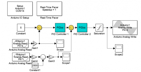
The proposed control scheme is implemented on Arduino mega 2560 for a DC micro-grid integrated buck converter as shown in Appendix B. Rapid control prototyping is utilized to program Arduino microcontroller from the Simulink environment as shown in Appendix A. The experiment is carried out under fixed load and also under load variations. The results obtained with proposed control scheme are than compared with classical SMC, PID and Fractional order PID controllers (FOPID). The control parameters are tabulated in Table 1 and Table 2, respectively.
Table 1. PID controller parameters
|
Controller |
Kp |
Ki |
Kd |
α |
|
PID voltage loop |
10 |
30 |
0.5 |
0 |
|
PID current loop |
5 |
12 |
0.5 |
0 |
|
FOPID voltage loop |
2 |
10 |
0.1 |
0.85 |
|
FOPID current loop |
1.5 |
5 |
0.1 |
0.85 |
Table 2. FSMC controller parameters
|
Controller |
c1 |
c2 |
c3 |
c4 |
K1 |
K2 |
α |
|
PID voltage loop |
5 |
2.5 |
3.2 |
1.3 |
0.5 |
1.25 |
0.2 |
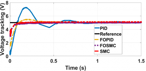
5.1 Voltage tracking under fixed load condition
Figures 3 and 4 show the voltage tracking and voltage error response of the system with different controllers under no load condition.
Figure 3. Voltage tracking response under fixed load
Figure 4. Voltage tracking error response under fixed load
The comparison of the voltage regulation response of the system under PID, FOPID, SMC and FSMC controllers are shown in Figure 3. The reference command signal is set to 5v. From the experimental results presented; the comparative data is tabulated in Table 3. From the results collected, it is concluded that the robust FSMC offers the desired performance in terms of rise time, settling time and steady state error when the system is connected to the fixed resistive load.
Table 3. Voltage tracking response
|
Controller |
Rise time (ms) |
Settling time (ms) |
Steady state error |
Overshoot (%) |
Peak voltage |
|
PID |
13.491 |
982.9 |
2.25 |
47.08 |
7.251 |
|
FOPID |
14.8 |
219.4 |
0.478 |
10.3 |
5.47 |
|
SMC |
7.499 |
35.6 |
0.059 |
1.94 |
0.59 |
|
FSMC |
7.199 |
33.6 |
0.049 |
1.74 |
0.49 |
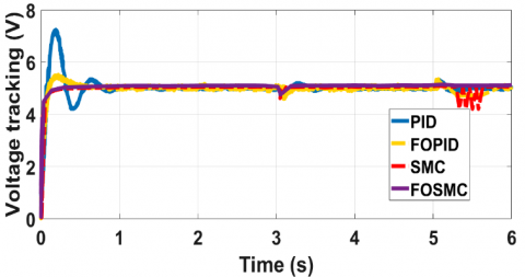
5.2 Voltage tracking response under load variations
In this section, the voltage tracking performance of the buck converter under load variations is compared with PID, FOPID, SMC and FSMC controllers. Reference command signal is selected as 5v. Initially a fixed 5 ohms resistive load is connected at the output of the buck converter. To check the robustness of all the above mentioned control schemes, two more resistors each carrying 5 ohms resistance are switched in parallel to the nominal load at t= 3sec and then switched off at t= 5sec. The voltage regulation and error response of buck converter system with PID, FOPID, SMC and FSMC controllers is shown in Figures 5 and 6 respectively. By observing the response of the system in all these cases between the time span between t= 3sec to 5sec, the following data points are collected.
For PID: The maximum error recorded is +0.21v to -0.3v. The steady state error is approaching zero at 3.5 sec and 5.4 sec respectively.
For FOPID: The maximum error recorded is +0.3v to -0.4v. The steady state error is approaching zero at 3.25 sec and 5.3 sec.
For FMSC: The maximum error recorded is +0.1v to -0.2v. The steady state error is approaching zero at 3.08 sec and 5.08 sec.
For SMC with saturation function: The maximum error recorded is +0.1v to -0.25v. The steady state error is approaching zero at 3.18 sec and 5.18 sec.
From the data comparison presented above it is concluded the in case of FSMC, the system states returns to steady state in the shortest time after when the system is subject to the load variations.
Figure 5. Voltage tracking response under load variations
Figure 6. Voltage tracking error response under load variations
Apart from the system response with load variations, the transient response of the system under all variants of control schemes is shown in Figure 5. By noting the voltage tracking response from time t=0 to 2 seconds, system with PID controller exhibits the largest error of +2v and -1v on both positive and negative sides of zero line, and also the settling time is around 1.5 sec. Similarly system with FOPID controller shows transient error of +1v and with improved settling time. From Figure 5, it is noted that FSMC controller shows superior transient and steady state performance under load variations.
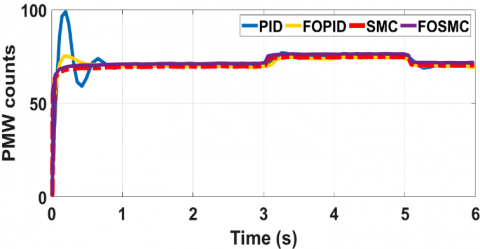
Figure 7. Control excitation response under load variations
Figure 8. Enlarged view of control signal under load variations
Figures 7 and 8 show the recorded control signal excitations for all variants of the discussed controllers. The control signal excitation is represented as pulse width modulation (PWM) register counts. Transient response of the control excitations for all variants of the discussed controllers is clear from Figure 7. In the event when load is varied, the enlarged view of the control excitations is shown in Figure 8. From the presented results it is clear that FSMC takes maximum counts of 76 and thus it gives the best transient and steady state response as obvious from Figures 5 and 6.
Fractional order sliding mode controller is derived and implemented for a DC micro-grid integrated buck converter system. The controller is tested under ideal and variable load conditions. From the results it is concluded that fractional order sliding mode controller offers superior performance in terms of rise time, settling time and percent overshoot as compared to classical SMC, PID, and fractional order PID controllers. In future the proposed control method will be studied with respect to the computational resource requirements when it is implemented over the microprocessor. Moreover different methods and modifications will be suggested to minimize its computational resource utilization for practical implementation over a microprocessor.
Appendix A: Simulink Block Diagrams
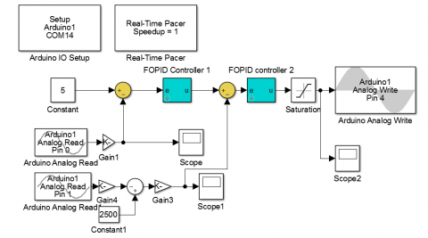
Figure A.1. PID based buck converter Simulink block diagram
Figure A.2. FPID based buck converter Simulink block diagram
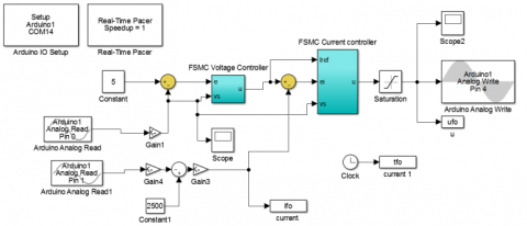
Figure A.3. FSMC based buck converter Simulink block diagram
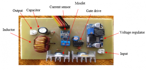
Figure A.4. Buck converter
Figure A.5. Experimental arrangement
Appendix B
Table B1. Buck converter and load bank parameters
|
Parameter |
Value |
Unit |
|
Source Voltage (Vi) |
18 |
Volt |
|
Output Voltage (Vo) |
5 |
Volt |
|
Switching frequency (Fsw) |
62.5 * 103 |
Hz |
|
Inductor |
32 * 10-6 |
Henry |
|
Capacitor (C) |
1000 * 10-6 |
Farad |
|
Power |
50 |
Watt |
|
Load current (maximum) |
10 |
Ampere |
|
Current ripple (Iripple) |
18 % |
Ampere |
|
Voltage ripple (Vripple) |
8 * 10-3 |
Volt |
|
Total time (ΔT) |
4.4 * 10-3 |
Second |
|
Load bank |
Four,5 ohms resistors are connected in parallel. Load changes are reflected by switching several resistors in parallel or disconnecting it |
ohms |
[1] Dragičević, T., Lu, X., Vasquez, J.C., Guerrero, J.M. (2015). DC microgrids—Part II: A review of power architectures, applications, and standardization issues. IEEE Transactions on Power Electronics, 31(5): 3528-3549. https://doi.org/10.1109/TPEL.2015.2464277
[2] Boroyevich, D., Cvetković, I., Dong, D., Burgos, R., Wang, F., Lee, F. (2010). Future electronic power distribution systems a contemplative view. In 2010 12th International Conference on Optimization of Electrical and Electronic Equipment, Basov, Romania, pp. 1369-1380. https://doi.org/10.1109/OPTIM.2010.5510477
[3] Dragicevic, T., Vasquez, J.C., Guerrero, J.M., Skrlec, D. (2014). Advanced LVDC electrical power architectures and microgrids: A step toward a new generation of power distribution networks. IEEE Electrification Magazine, 2(1): 54-65. https://doi.org/10.1109/MELE.2013.2297033
[4] Kakigano, H., Miura, Y., Ise, T. (2010). Low-voltage bipolar-type DC microgrid for super high quality distribution. IEEE Transactions on Power Electronics, 25(12): 3066-3075. https://doi.org/10.1109/TPEL.2010.2077682
[5] Ito, Y., Zhongqing, Y., Akagi, H. (2004). DC microgrid based distribution power generation system. In the 4th International Power Electronics and Motion Control Conference, 2004. IPEMC 2004, 3: 1740-1745.
[6] Kwasinski, A., Krein, P.T. (2005). A microgrid-based telecom power system using modular multiple-input dc-dc converters. In INTELEC 05-Twenty-Seventh International Telecommunications Conference, Berlin, Germany, pp. 515-520. https://doi.org/10.1109/INTLEC.2005.335152
[7] Kakigano, H., Miura, Y., Ise, T., Uchida, R. (2006). DC micro-grid for super high quality distribution—System configuration and control of distributed generations and energy storage devices. In 2006 37th IEEE Power Electronics Specialists Conference, Jeju, South Korea, pp. 1-7. https://doi.org/10.1109/pesc.2006.1712250
[8] Salomonsson, D., Soder, L., Sannino, A. (2007). An adaptive control system for a DC microgrid for data centers. In 2007 IEEE Industry Applications Annual Meeting, New Orleans, LA, USA. https://doi.org/10.1109/07IAS.2007.364
[9] Biczel, P. (2007). Power electronic converters in dc microgrid. In 2007 Compatibility in Power Electronics, Gdansk, Poland, pp. 1-6. https://doi.org/10.1109/CPE.2007.4296505
[10] Valenciaga, F., Puleston, P.F. (2005). Supervisor control for a stand-alone hybrid generation system using wind and photovoltaic energy. IEEE Transactions on Energy Conversion, 20(2): 398-405. https://doi.org/10.1109/TEC.2005.845524
[11] Knight, A.M., Peters, G.E. (2005). Simple wind energy controller for an expanded operating range. IEEE Transactions on Energy Conversion, 20(2): 459-466. https://doi.org/10.1109/TEC.2005.847995
[12] Ekneligoda, N.C., Weaver, W.W. (2013). A game theoretic bus selection method for loads in multibus DC power systems. IEEE Transactions on Industrial Electronics, 61(4): 1669-1678. https://doi.org/10.1109/TIE.2013.2267702
[13] Shafiee, Q., Dragičević, T., Vasquez, J.C., Guerrero, J.M. (2014). Hierarchical control for multiple DC-microgrids clusters. IEEE Transactions on Energy Conversion, 29(4): 922-933. https://doi.org/10.1109/TEC.2014.2362191
[14] Park, J.D., Candelaria, J., Ma, L., Dunn, K. (2013). DC ring-bus microgrid fault protection and identification of fault location. IEEE Transactions on Power Delivery, 28(4): 2574-2584. https://doi.org/10.1109/TPWRD.2013.2267750
[15] Cupelli, M., Zhu, L., Monti, A. (2014). Why ideal constant power loads are not the worst case condition from a control standpoint. IEEE Transactions on Smart Grid, 6(6): 2596-2606. https://doi.org/10.1109/TSG.2014.2361630
[16] AL-Nussairi, M.K., Bayindir, R., Padmanaban, S., Mihet-Popa, L., Siano, P. (2017). Constant power loads (cpl) with microgrids: Problem definition, stability analysis and compensation techniques. Energies, 10(10): 1656. https://doi.org/10.3390/en10101656
[17] Asghar, M., Khattak, A., Rafiq, M.M. (2017). Comparison of integer and fractional order robust controllers for DC/DC converter feeding constant power load in a DC microgrid. Sustainable Energy, Grids and Networks, 12: 1-9. https://doi.org/10.1016/j.segan.2017.08.003
[18] Karlsson, P., Svensson, J. (2003). DC bus voltage control for a distributed power system. IEEE Transactions on Power Electronics, 18(6): 1405-1412. https://doi.org/10.1109/TPEL.2003.818872
[19] Balog, R.S. (2006). Autonomous local control in distributed DC power systems. University of Illinois at Urbana-Champaign.
[20] Rahimi, A.M., Emadi, A. (2009). Active damping in DC/DC power electronic converters: A novel method to overcome the problems of constant power loads. IEEE Transactions on Industrial Electronics, 56(5): 1428-1439. https://doi.org/10.1109/TIE.2009.2013748
[21] Johnson, B.K., Lasseter, R.H., Alvarado, F.L., Adapa, R. (1993). Expandable multiterminal DC systems based on voltage droop. IEEE Transactions on Power Delivery, 8(4): 1926-1932. https://doi.org/10.1109/61.248304
[22] Koutroulis, E., Kalaitzakis, K. (2006). Design of a maximum power tracking system for wind-energy-conversion applications. IEEE Transactions on Industrial Electronics, 53(2): 486-494. https://doi.org/10.1109/TIE.2006.870658
[23] Subudhi, B., Pradhan, R. (2012). A comparative study on maximum power point tracking techniques for photovoltaic power systems. IEEE Transactions on Sustainable Energy, 4(1): 89-98. https://doi.org/10.1109/TSTE.2012.2202294
[24] Dragicevic, T., Guerrero, J.M., Vasquez, J.C., Skrlec, D. (2014). Supervisory control of an adaptive-droop regulated DC microgrid with battery management capability. IEEE Trans. Power Electron., 29(2): 695-706. https://doi.org/10.1109/TVT.2006.877483
[25] Emadi, A., Khaligh, A., Rivetta, C.H., Williamson, G.A. (2006). Constant power loads and negative impedance instability in automotive systems: definition, modeling, stability, and control of power electronic converters and motor drives. IEEE Transactions on Vehicular Technology, 55(4): 1112-1125. https://doi.org/10.1109/TVT.2006.877483
[26] Forsyth, A.J., Mollov, S.V. (1998). Modeling and control of DC-DC Converters. Power Engineering, 12(5): 229-236. https://doi.org/10.1049/pe:19980507
[27] Mattavelli, P., Rossetto, L., Spiazzi, G. (1995). Small-signal analysis of DC-DC converters with sliding mode control. In Proceedings of 1995 IEEE Applied Power Electronics Conference and Exposition-APEC'95, 1: 153-159. https://doi.org/10.1109/APEC.1995.469014
[28] Matas, J., Vicuna, L.G., Lopez, O., Lopez, M., Castilla, M. (1999). Sliding-LQR based control of dc-dc converters. In European Power Electronics Conference 99, Lausanne, pp. 7-9.
[29] Ananda Natarajan, R., Chidambaram, M., Jayasingh, T. (2012). Limitation of a PI controller for first-order nonlinear process with dead time. ISA Transaction, 45(2): 185-199. https://doi.org/10.1016/S0019-0578(07)60189-X
[30] Abbas, G., Farooq, U., Gu, J., Asad, M.U. (2014). Application of a robust fuzzy logic controller with smaller rule base to a DC-DC buck converter. In 2014 International Conference on Open Source Systems & Technologies, pp. 70-75. https://doi.org/10.1109/ICOSST.2014.7029323
[31] Gupta, T., Boudreaux, R.R., Nelms, R.M., Hung, J.Y. (1997). Implementation of a fuzzy controller for DC-DC converters using an inexpensive 8-b microcontroller. IEEE transactions on Industrial Electronics, 44(5): 661-669. https://doi.org/10.1109/41.633467
[32] So, W., Tse, C.K., Lee, Y. (1996). Development of a FLC for DC/DC converters. IEEE Trans. Power Electron, 11(1): 24-32.
[33] Guldemir, H. (2011). Study of sliding mode control of DC-DC buck converter. Energy and Power Engineering, 3(04): 401-406. https://doi.org/10.4236/epe.2011.34051
[34] Wu, B., Yang, J., Wang, J., Li, S. (2014). Extended state observer based control for DC-DC buck converters subject to mismatched disturbances. In Proceedings of the 33rd Chinese Control Conference, pp. 8080-8085. https://doi.org/10.1109/ChiCC.2014.6896352
[35] Olalla, C., Queinnec, I., Leyva, R., El Aroudi, A. (2011). Robust optimal control of bilinear DC–DC converters. Control Engineering Practice, 19(7): 688-699. https://doi.org/10.1016/j.conengprac.2011.03.004
[36] Emadi, A., Ehsani, M. (2000). Negative impedance stabilizing controls for PWM DC-DC converters using feedback linearization techniques. In Collection of Technical Papers. 35th Intersociety Energy Conversion Engineering Conference and Exhibit (IECEC)(Cat. No. 00CH37022), 1: 613-620. https://doi.org/10.1109/IECEC.2000.870842
[37] Komurcugil, H. (2012). Adaptive terminal sliding-mode control strategy for DC–DC buck converters. ISA Transactions, 51(6): 673-681. https://doi.org/10.1016/j.isatra.2012.07.005
[38] Tan, S.C., Lai, Y.M., Tse, C.K., Cheung, M.K. (2006). Adaptive feedforward and feedback control schemes for sliding mode controlled power converters. IEEE Transactions on Power Electronics, 21(1): 182-192. https://doi.org/10.1109/TPEL.2005.861191
[39] Wang, J., Li, S., Yang, J., Wu, B., Li, Q. (2015). Extended state observer-based sliding mode control for PWM-based DC–DC buck power converter systems with mismatched disturbances. IET Control Theory & Applications, 9(4): 579-586. https://doi.org/10.1049/iet-cta.2014.0220
[40] Delghavi, M.B., Shoja-Majidabad, S., Yazdani, A. (2016). Fractional-order sliding-mode control of islanded distributed energy resource systems. IEEE Transactions on Sustainable Energy, 7(4): 1482-1491. https://doi.org/10.1109/TSTE.2016.2564105
[41] Matignon, D. (1998). Stability properties for generalized fractional differential systems. In ESAIM: Proceedings, 5: 145-158. http://dx.doi.org/10.1051/proc:1998004
[42] Aghababa, M.P. (2014). A lyapunov-based control scheme for robust stabilization of fractional chaotic systems. Nonlinear Dynamics, 78(3): 2129-2140. https://doi.org/10.1007/s11071-014-1594-8
[43] Li, C., Deng, W. (2007). Remarks on fractional derivatives. Applied Mathematics and Computation, 187(2): 777-784. https://doi.org/10.1016/j.amc.2006.08.163
[44] Calderon, A.J., Vinagre, B.M., Feliu, V. (2003). Linear fractional order control of a DC-DC buck converter. In 2003 European Control Conference (ECC), pp. 1292-1297. https://doi.org/10.23919/ECC.2003.7085139
[45] Monje, C.A., Chen, Y., Vinagre, B.M., Xue, D., Feliu-Batlle, V. (2010). Fractional-order systems and controls: fundamentals and applications. Springer Science & Business Media. XVI, 415. https://doi.org/10.1007/978-1-84996-335-0
[46] Ullah, N., Ullah, A., Ibeas, A., Herrera, J. (2017). Improving the hardware complexity by exploiting the reduced dynamics-based fractional order systems. IEEE Access, 5: 7714-7723. https://doi.org/10.1109/ACCESS.2017.2700439
[47] Li, Y., Chen, Y., Podlubny, I. (2010). Stability of fractional-order nonlinear dynamic systems: Lyapunov direct method and generalized Mittag–Leffler stability. Computers & Mathematics with Applications, 59(5): 1810-1821. https://doi.org/10.1016/j.camwa.2009.08.019
[48] Monje, C.A., Vinagre, B.M., Feliu, V., Chen, Y. (2008). Tuning and auto-tuning of fractional order controllers for industry applications. Control Engineering Practice, 16(7): 798-812. https://doi.org/10.1016/j.conengprac.2007.08.006