Rehab Ali Khudair* | Ameera N. Alkiffai | Athraa Neamah Albukhuttar
© 2020 IIETA. This article is published by IIETA and is licensed under the CC BY 4.0 license (http://creativecommons.org/licenses/by/4.0/).
OPEN ACCESS
In this article, a fuzzy Elzaki transform (FZT) is discussed in the context of highly-generalized differentiability concepts, where a new formula of fuzzy derivatives for the fuzzy Elzaki transform is derived as well. It shows the applicability of this interesting fuzzy transform for solving differential equations with constant coefficients also for its computational power. Since ordinary linear equations are mostly used in physical fields, the motion of a mass on a vibrating spring problem is solved by using this kind of fuzzy Elzaki transform.
fuzzy Elzaki transform, Sumudu transform, the motion of a mass, vibrating spring equation
There is no doubt that most mathematical equations, including multiple variables or constant coefficients, and their derivatives deal with real-life phenomena. Various aspects of physics, engineering, and biology have been adapted to common differential equations, which are indicators of the crucial role of partial differential equations in modeling problems. [1] Analytical and numerical methods have been utilized by numerous researchers to solve common differential equations [2, 3]. Even so, these equations (ODEs) are limited to dealing with some important cases, such as the modeling of a certain dynamic phenomenon using (ODEs) where it is not always accurate. In addition to inadequate data and understanding of the dynamic system, fuzziness in the initial values may provide an explanation for this.
On the other hand, in operational calculations that use solving (ODEs), integral transforms constitute critical tools and can be useful. It seems that integrated transformations convert the original complicated function into an easier-to-resolve new function. In this regard, the Fourier transform can consider as the first integral transform then followed by Laplace, Mellin, and wavelet transform [4]. Fuzzy transforms such as Laplace and Sumudu were then applied to solve ordinary linear fuzzy differential equation [5-7]. Indeed, fuzzy transform not just solve (ODEs) but also fractional nonlinear partial differential equations, fractional ordinary differential equations, and system of linear partial or ordinary differential equations [8-11]. Fuzzy transform was proposed as a pilot fuzzy approximation approach to applying in unusual application fields such as numerical solutions of (ODEs) [12].
Bulut et al. [13] employed the Sumudu transform to solve nonhomogeneous fractional ordinary differential equations. The findings showed the fact that the Sumudu transform can be employed to solve many problems of applied sciences. Yang and Hou [14] proofed that The Laplace decomposition method is a precise technique to deal with both linear and nonlinear fractional integrodifferential equations. In the same regard, Mohammed [15] presented numerical examples and used the least-squares method to solve linear fractional integro-differential equations.
Jena and Chakraverty [16] introduced a hybrid technique to solve the Navier–Stokes equation. The findings showed that the proposed method is accurate, successful, and simple to use for various science and engineering-related issues. Verma and Alam [17] presented some of the examples in the electric circuit and proved that the technique of Elzaki transform was very strong in simultaneous differential equations. In the same regard, Suleman et al. [18] compared Elzaki 's transform with other conventional methods and found it to be versatile and has flexible efficiency. Ziane et al. [19] evaluated Elzaki 's transition to solve nonlinear partial differential equations with time-fractional derivative and reported that the technique quite successful for such problems. Singh and Sharma [20] argued that the transformation of Elzaki and its properties could be attributed to the transformation of Laplace. They employed the technique on nonlinear homogeneous and non-homogenous fractional and showed that methodologies suggested solving this kind of complex equation were effective, simple, and highly accurate. Ige et al. [21] combined the Elzaki transform method and Adomian polynomials to solve Klein-Gordon equations. The results are consistent with the results of previous studies regarding the accuracy and efficiency of the Elzaki transform. Khalouta and Kadem [22] employed a mixed Elzaki transform and the projected differential transformation method and reported that the technique was reliable compared to the traditional techniques.
Lately, to solve the linear system, Tarig M. Elzaki and Salih M. Elzaki produced a new integral transformation, it was Elzaki transform [23], which then used by Tarig [24] to solve common differential equations with more details. For the same purpose, Adam [25] conducted a comparative investigation between two methods, i.e. Adomain Decomposition and Elzaki Transform, and reported that both techniques were powerful and efficient. Khalid et al. [26] employed Elzaki transform to solve non-homogeneous fractional by using Matlab and MathWork.
Note that, the concept of derivative proposed by Bede and Gal [27] is based on the Hukuhara difference that co-called by "generalized Hukuhara differentiability”. Moreover, the existence and uniqueness of a “solution of fuzzy initial value” problem in higher-order using the “classical form of Hukuhara differentiability has been” represented by Georgiou et al. [28]. The motion of a mass on a vibrating spring, which represents a real problem which solving by this new technique.
In this article, in-state dealing with classical kinds of (ODEs), we submit a new method for solving (FODEs) using (FZT). The current manuscript is partition as shown below: Section 1, here we review some of the fundamental definitions of the concept of a fuzzy number. Section 2, we represented fuzzy Elzaki transform definition (FZT) beside some related theorems and their proofs. Section 3, the connection between fuzzy Sumudu transform (FST) and (FZT) is discussed by theorems concerning the (FZT) to solve (ODEs). Section 4, as a real-life problem, the motion of a mass on a spring is discussed as an application for fuzzy Elzaki transform.
2.1 Fuzzy number [3]
A fuzzy number $\psi$ in parametric form is a pair $(\underline{\psi}, \bar{\psi})$ of functions $\underline{\psi}(\eta), \bar{\psi}(\eta), 0 \leq \eta \leq 1,$ that meets the requirements as follows:
1- $\underline{\psi}(\eta)$ is a bounded non-decreasing left continuous function in (0,1] while right continuous at 0.
2- $\bar{\psi}(\eta)$ is a bounded non-increasing left continuous function in (0,1], and right continuous at 0.
3- $\underline{\psi}(\eta) \leq \bar{\psi}(\eta), 0 \leq \eta \leq 1$.
2.2 Operations of fuzzy number [3]
Let $\psi=(\underline{\psi}(\eta), \bar{\psi}(\eta)), 0 \leq \eta \leq 1$ and $\theta=(\underline{\theta}(\eta), \bar{\theta}(\eta))$, $\eta>0$ be an arbitrary constant, we can realize addition $\psi \oplus \theta$ subtraction $\psi \ominus \theta$ and scalar multiplication by $\propto$ as:
(a) Addition: $\psi \oplus \theta=(\underline{\psi}(\eta)+\underline{\theta}(\eta), \bar{\psi}(\eta)+\bar{\theta}(\eta))$
(b) Subtraction $\psi \ominus \theta=(\underline{\psi}(\eta)-\underline{\theta}(\eta), \bar{\psi}(\eta)-\bar{\theta}(\eta))$
(c) Scalar multiplication $\propto \odot \psi=\left\{\begin{array}{l}(\propto \underline{\psi}, \alpha \bar{\psi}) \propto \geq 0 \\ (\propto \bar{\psi}, \alpha \underline{\psi}) \propto<0\end{array}\right\}$
2.3 Fuzzy values for functions of the first derivative [29]
Let $\xi: R \rightarrow E$ be a function and denote $\xi(\tau)=$ $(\underline \xi(\tau ; \eta), \bar{\xi}(\tau ; \eta))$ for each $r \in[0,1]$ Then
1-If $\xi$ is no.1, then $\xi(\tau ; \eta)$ and $\bar{\xi}(\tau ; \eta)$ are differentiable functions and $\xi^{\prime}(\tau)=(\underline\xi(\tau ; \eta), \bar{\xi}(\tau ; \eta))$.
2-If $\xi$ is no.2, then $\underline\xi(\tau ; \eta)$ and $\bar{\xi}(\tau ; \eta)$ are differentiable functions and $\xi^{\prime}(\tau)=(\bar{\xi}(\tau ; \eta), \underline\xi(\tau ; \eta))$.
2.4 Fuzzy values for functions of the nth derivatives [30]:
Suppose that $\beta(\tau), \beta^{\prime}(\tau), \ldots, \beta^{n-1}(\tau)$ are differential fuzzy valued functions such that $\beta^{(i 1)}(\tau), \beta^{(i 2)}(\tau), \ldots, \beta^{(i m)}(\tau)$ are no.2 functions for $0 \leq i_{1}<i_{2}<i_{3}<\ldots<i_{m} \leq n-1$ and $\beta^{p}(\tau)$ is no.1 for $p \neq i_{j}, j=1,2,3, \ldots, m$ and if $\eta-$ cut representation of fuzzy $-$ value function $\beta(\tau)$ is denoted by $\beta(\tau)=(\underline{\beta}(\tau, \eta), \bar{\beta}(\tau, \eta)),$ then:
a. If $m$ is an E.N, then $\beta^{(n)}(\tau)=\left(\underline{\beta}^{(n)}(\tau, \eta), \bar{\beta}^{(n)}(\tau, \eta)\right)$.
b. If $m$ is an O.N, then $\quad \beta^{(n)}(\tau)=\left(\bar{\beta}^{(n)}(\tau, \eta), \underline{\beta}^{(n)}(\tau, \eta)\right)$.
2.5 Fuzzy Sumudu transform for fuzzy nth derivatives [31, 32]
Suppose the $\beta(\tau), \beta^{\prime}(\tau), \ldots, \beta^{n-1}(\tau)$ are continuous fuzzyvalue function on $[0, \infty)$ and of exponential order that $\beta^{n}(\tau)$ is piecewise continuous fuzzy- valued function on $[0, \infty)$. Let $\beta^{(i 1)}(\tau), \beta^{(i 2)}(\tau), \ldots, \beta^{(i m)}(\tau)$ are no. 2 function for $0 \leq i_{1}<$ $i_{2}<i_{3}<\ldots<i_{m} \leq n-1$ and $\beta^{p}(\tau)$ is no.1 function $p \neq$ $i_{j}, j=1,2,3, \ldots, m$ and, $\beta(\tau)=(\beta(\tau, \eta), \bar{\beta}(\tau, \eta)),$ then
1. If $m$ is an E.N, we have $S\left[\beta^{n}(\tau)\right]=\frac{\psi(u)}{u^{n}} \ominus \frac{\beta(0)}{u^{n}} \otimes$ $\sum_{k=1}^{n-1} \frac{1}{u^{n-k}} \beta^{k}(0)$.
Such that
$\otimes=\left\{\begin{array}{l}\ominus \text { If the no. } 2 \text { functions } \beta^{i}(\tau), \text { provided } i<k \text { is } 0 . \mathrm{N} \\ -\text { If the no. } 2 \text { functions } \beta^{i}(\tau), \text { provided } i<k \text { is E. } \mathrm{N}\end{array}\right.$
2. If m is an O.N, we have
$S\left[\beta^{n}(\tau)\right]=-\frac{\beta(0)}{u^{n}} \ominus\left(-\frac{\Psi(u)}{u^{n}}\right) \otimes \sum_{k=1}^{n-1} \frac{1}{u^{n-k}} \beta^{k}(0)$
Such that
$\otimes=\left\{\begin{array}{l}\ominus \text { If the no. } 2 \text { functions } \beta^{i}(\tau), \text { provided } i<k \text { is } 0 . \mathrm{N} \\ -\text { If the no. } 2 \text { functions } \beta^{i}(\tau), \text { provided } i<k \text { is E. } \mathrm{N}\end{array}\right.$
3.1 Fuzzy Elzaki transform
let $\psi: R \rightarrow E(R)$ be continuous fuzzy -valued function, consider that $u^{2} \psi(u \tau) e^{-\tau} d \tau$ is improper fuzzy Riemannintegral on $[0, \infty),$ then $u^{2} \int_{0}^{\infty} \psi(u \tau) e^{-\tau} d \tau$ is named fuzzy Elzaki transform which is define by $\Phi(u)=E[\psi(\tau)]=$ $u^{2} \int_{0}^{\infty} \psi(u \tau) e^{-\tau} d \tau, k_{1}<u<k_{2},$ then we get:
$u^{2} \int_{0}^{\infty} \psi(u \tau) e^{-\tau} d \tau=$ $\left[u^{2} \int_{0}^{\infty} \underline{\psi}(u \tau) e^{-\tau} d \tau, u^{2} \int_{0}^{\infty} \bar{\psi}(u \tau) e^{-\tau} d \tau\right],$ by classical $\mathrm{Elzaki}$ transform, we have:
$e[\underline{\psi}(\tau, \eta)]=u^{2} \int_{0}^{\infty} \underline{\psi}(u \tau) e^{-\tau} d \tau$,
$e[\bar{\psi}(\tau, \eta)]=u^{2} \int_{0}^{\infty} \bar{\psi}(u \tau) e^{-\tau} d \tau$.
Finally, we get: $E[\psi(\tau)]=(e[\underline{\psi}(\tau ; \eta)], e[\bar{\psi}(\tau ; \eta)])$.
3.2 Linear property
Let $\psi, \theta: \Re \rightarrow E(\Re)$ be two continuous fuzzy functions, assume that $b_{1}$ and $b_{2}$ random constants, after that:
$E\left[\left(b_{1} \quad \odot \psi(\tau)\right) \oplus\left(b_{2} \odot \theta(\tau)\right)\right]=\left(b_{1} \quad \odot E(\psi(\tau)) \oplus\right.$$\left(b_{2} \odot E(\theta(\tau))\right.$
Proof: $\quad$ let $\quad \psi(\tau)=(\underline{\psi}(\tau ; \eta), \bar{\psi}(\tau ; \eta)), \theta(\tau)=$ $(\underline{\theta}(\tau ; \eta), \bar{\theta}(\tau ; \eta))$
Form definition (3.1), we obtain
$e\left(\left[b_{1} \underline{\psi}(\tau)\right]+\left[b_{2} \underline{\theta}(\tau)\right]\right)$
$=u^{2} \int_{0}^{\infty} b_{1} \underline{\psi}(u \tau) e^{-\tau} d \tau$
$+u^{2} \int_{0}^{\infty} b_{2} \underline{\theta}(u \tau) e^{-\tau} d \tau$
$=b_{1} \int_{0}^{\infty} u^{2} \underline{\psi}(u \tau) e^{-\tau} d \tau$
$+b_{2} \int_{0}^{\infty} u^{2} \underline{\theta}(u \tau) e^{-\tau} d \tau$
$=b_{1} e[\underline{\psi}(\tau)]+b_{2} e[\underline{\theta}(\tau)]$
And
$e\left(\left\lceil b_{1} \bar{\psi}(\tau)\right]+\left[b_{2} \bar{\theta}(\tau)\right]\right)$
$=u^{2} \int_{0}^{\infty} b_{1} \bar{\psi}(u \tau) e^{-\tau} d \tau$
$+u^{2} \int_{0}^{\infty} b_{2} \bar{\theta}(u \tau) e^{-\tau} d \tau$
$=b_{1} \int_{0}^{\infty} u^{2} \bar{\psi}(u \tau) e^{-\tau} d \tau$
$+b_{2} \int_{0}^{\infty} u^{2} \bar{\theta}(u \tau) e^{-\tau} d \tau$
$=b_{1} e[\bar{\psi}(\tau)]+b_{2} e[\bar{\theta}(\tau)]$
Thus,
$\left(b_{1} \odot E(\psi(\tau)) \oplus\left(b_{2} \odot E(\theta(\tau))\right.\right.$.
3.3 Change of scale property
Consider $\psi: \Re \rightarrow E(\Re)$ be a continuous fuzzy function and $b$ is a random constant then, $E[\psi(b \tau)]=\Phi(b \tau)$.
Proof: We have:
$\psi(\tau)=(\underline{\psi}(b \tau ; \alpha), \bar{\psi}(b \tau ; \alpha))=(e[\underline{\psi}(b \tau ; \alpha)], e[\bar{\psi}(b \tau ; \alpha)])$
$=\left(u^{2} \int_{0}^{\infty} \underline{\psi}(b u \tau, \alpha) d \tau, u^{2} \int_{0}^{\infty} \bar{\psi}(b u \tau, \alpha) d \tau\right)=\Phi(b \tau)$
4.1 Connection between fuzzy Sumudu and Elzaki transforms
Let $\psi(\tau)$ be a continuous fuzzy - value function, if $\Psi(u)$ is a fuzzy the Sumudu of $\psi(\tau)$ and $\Phi(u)$ is the fuzzy Elzaki transform of $\psi(\tau)$ then $\Phi(u)=u^{2} \Psi(u)$
Proof: let $\psi(\tau) \in E(\Re)$ then $u \in k_{1}, k_{2} .$ Form definition (3.1), we get
$\begin{aligned} \Phi(u)=E[\psi(\tau)] &=\left(\begin{array}{c}u^{2} \int_{0}^{\infty} \frac{\psi(u \tau, \eta) e^{-\tau} d \tau}{-} \\ u^{2} \int_{0}^{\infty} \bar{\psi}(u \tau, \eta) e^{-\tau} d \tau\end{array}\right), \Phi(u) \\=u^{2} &\left(\begin{array}{l}\int_{0}^{\infty} \frac{\psi(u \tau, \eta) e^{-\tau} d \tau}{\psi} \\ \int_{0}^{\infty} \bar{\psi}(u \tau, \eta) e^{-\tau} d \tau\end{array}\right) \Phi(u)=u^{2} \Psi(u) \end{aligned}$
4.2 The first derivative to fuzzy Elzaki transform
Let $\psi: R \rightarrow E(R)$ be continuous fuzzy -value function and $\psi$ is the primitive of $\psi^{\prime}$ on $[0, \infty),$ and
1. If $\psi(\tau)$ is no.1, $E\left[\psi^{\prime}(\tau)\right]=\frac{\Phi(u)}{u} \ominus u \psi(0)$.
2. If $\psi(\tau)$ is no.2, $E\left[\psi^{\prime}(\tau)\right]=-u \psi(0) \ominus\left(-\frac{\Phi(u)}{u}\right)$.
Proof: $(1),$ since $\psi(\tau)$ is no. $1,$ then by theorem $(2.1 .4)(\mathrm{a})$ we get:
$\psi^{\prime}(\tau)=\left(\underline{\psi^{\prime}}(\tau), \overline{\psi^{\prime}}(\tau)\right)$
Therefore, we obtain
$E\left[\psi^{\prime}(\tau)\right]=E\left(\underline{\psi}^{\prime}(\tau), \bar{\psi}^{\prime}(\tau)\right)=\left(e\left[\underline{\psi}^{\prime}(\tau)\right], e\left[\bar{\psi}^{\prime}(\tau)\right]\right)$.
From Elzaki transform, we get
$e\left[\overline{\psi^{\prime}}(\tau)\right]=\frac{\Phi(u)}{u}-u \bar{\psi}(0)$
$e\left[\underline{\psi^{\prime}}(\tau)\right]=\frac{\Phi(u)}{u}-u \underline{\psi}(0)$ (1)
Since $\psi(\tau)$ is no.1, then by theorem (2.4) (a) we get,
$\psi(0)=(\underline{\psi}(0, \alpha), \bar{\psi}(0, \alpha))$,
then the Eq. (1) become
$E\left[\psi^{\prime}(\tau)\right]=\left(\frac{e[\underline{\psi}(\tau, \alpha]}{u}-u \underline{\psi}(0, \alpha), \frac{e[\bar{\psi}(\tau, \alpha]}{u}-u \bar{\psi}(0, \alpha)\right)$ $=\frac{\Phi(u)}{u} \ominus u \psi(0)$
Now to prove (2), since $\psi(\tau)$ is no.2, then by theorem (2.4) (b), we get:
$\psi^{\prime}(\tau)=\left(\overline{\psi^{\prime}}(\tau), \underline{\psi^{\prime}}(\tau)\right)$
Therefore, we obtain
$\left.E\left[\psi^{\prime}(\tau)\right]=E\left(\overline{\psi^{\prime}}(\tau), \underline{\psi}^{\prime}(\tau)\right)=(e [\underline{\psi} ^{\prime}(\tau)], e\left[\bar{\psi}^{\prime}(\tau)\right]\right)$.
From Elzaki transform, we get
$e\left[\overline{\psi^{\prime}}(\tau)\right]=\frac{\Phi(u)}{u}-u \bar{\psi}(0)$
$e\left[\underline{\psi}^{\prime}(\tau)\right]=\frac{\Phi(u)}{u}-u \underline{\psi}(0)$ (2)
Since $\psi(\tau)$ is no.2, then by theorem (2.4) (b) we get, $\psi(0)=(\bar{\psi}(0, \alpha), \underline{\psi}(0, \alpha))$, then the Eq. (1) become
$\left.E\left[\psi^{\prime}(\tau)\right]=\left(\frac{e[\underline{\psi}(\tau, \alpha]}{u}-u \underline{\psi}(0, \alpha), \frac{e[\bar{\psi}(\tau, \alpha]}{u}-u \bar{\psi}(0, \alpha)\right)\right)$ $=-u \psi(0) \ominus\left(-\frac{\Phi(u)}{u}\right)$
4.3 The second derivative to fuzzy Elzaki transform
let $\psi(\tau)$ and $\psi^{\prime}(\tau)$ are continuous fuzzy-value function on $[0, \infty)$ and $\psi^{\prime \prime}(\tau)$ is the piecewise continuous fuzzy $-$ valued function on $[0, \infty),$ then
1. If $\psi(\tau)$ and $\psi^{\prime}(\tau)$ no.2, then $E\left[\psi^{\prime \prime}(\tau)\right]=\frac{\Phi(u)}{u} \ominus \psi(0) \ominus$ $u \psi^{\prime}(0)$
2. If $\psi(\tau)$ is no.1 and $\psi^{\prime}(\tau)$ is no.2, then $E\left[\psi^{\prime \prime}(\tau)\right]=$ $-\psi(0) \ominus\left(-\frac{\Phi(u)}{u}\right)-u \psi^{\prime}(0)$
3. If $\psi^{\prime}(\tau)$ is no.1 and $\psi(\tau)$ is no.2, then $E\left[\psi^{\prime \prime}(\tau)\right]=$ $-\psi(0) \ominus\left(-\frac{\Phi(u)}{u}\right) \theta u \psi^{\prime}(0)$
4. If $\psi(\tau)$ and $\psi^{\prime}(\tau)$ are no.1, then $E\left[\psi^{\prime \prime}(\tau)\right]=\frac{\Phi(u)}{u} \ominus$ $u \psi(0)-\psi^{\prime}(0)$
Proof: we prove (2); since $\psi(\tau)$ is no.1 and $\psi^{\prime}(\tau)$ is no.2, then by theorem (2.5) (b), we get
$\psi^{\prime \prime}(\tau)=\left[\overline{\psi^{\prime \prime}}(\tau), \underline{\psi^{\prime \prime}}(\tau)\right]$
where,
$E\left[\psi^{\prime}(\tau)\right]=E\left[\overline{\psi^{\prime \prime}}(\tau), \underline{\psi^{\prime \prime}}(\tau)\right]=\left(e\left[\overline{\psi^{\prime \prime}}(\tau)\right], e\left[\underline{\psi^{\prime \prime}}(\tau)\right]\right)$
From the Elzaki transform, we get
$e\left(\overline{\psi^{\prime \prime}}(\tau, \eta)=\frac{e[\bar{\psi}(\tau, \alpha]}{u}-\bar{\psi}(0)-u \bar{\psi}^{\prime}(0)\right.$
$e\left(\underline{\psi^{\prime \prime}}(\tau, \eta)=\frac{e[\underline{\psi}(\tau, \alpha]}{u}-\underline{\psi}(0)-u \underline{\psi}^{\prime}(0)\right.$ (3)
Since $\psi(\tau)$ is no.1 and $\psi^{\prime}(\tau)$ is no.2, then by theorem (2.4) (a) we get
$\psi(0)=\lceil\underline{\psi}(0, \eta), \bar{\psi}(0, \eta)], \psi^{\prime}(0)=\left\lceil\overline{\psi^{\prime}}(0, \eta), \underline{\psi}^{\prime}(0, \eta)\right]$
then the Eq. (3) become
$E\left[\psi^{\prime \prime}(\tau)\right]=\left[\frac{e[\bar{\psi}(\tau, \alpha]}{u}-\bar{\psi}(0)-u \bar{\psi}^{\prime}(0), \frac{e[\underline{\psi}(\tau, \alpha]}{u}-\underline{\psi}(0)\right.$
$\left.-u \underline{\psi}^{\prime}(0)\right] E\left[\psi^{\prime \prime}(\tau)\right]$$=-\psi(0) \ominus\left(-\frac{\Phi(u)}{u}\right)-u \psi^{\prime}(0)$
4.4 Fuzzy Elzaki transform for fuzzy nth derivatives
Suppose that $\psi(\tau), \psi^{\prime}(\tau), \ldots, \psi^{n-1}(\tau)$ are continuous fuzzy- value function on $[0, \infty)$ and of exponential order that $\psi^{n}(\tau)$ is piecewise continuous fuzzy- valued function on $[0, \infty) .$ Let $\psi^{i_{1}}(\tau), \psi^{i_{2}}(\tau), \ldots, \psi^{i_{m}}(\tau)$ are no.2 function for $0 \leq i_{1}<i_{2}<i_{3}<\ldots<i_{m} \leq n-1 \quad$ and $\quad \psi^{p}(\tau) \quad$ is no.1 function $p \neq i_{j}, j=1,2,3, \ldots, m, \psi(\tau)=(\underline{\psi}(\tau, \eta), \bar{\psi}(\tau, \eta))$ and 1-If $m$ is an E.N, we have $\Phi_{n}(u)=\left\lceil\frac{E[\psi(\tau)]}{u^{n}} \ominus \frac{\psi(0)}{u^{n-2}} \otimes \sum_{k=1}^{n-1} \frac{1}{u^{n-k-2}} \psi^{k}(0)\right]$
Such that
$\otimes=\left\{\begin{array}{l}\ominus \text { If the no. } 2 \text { functions } \psi^{l}(\tau), \text { provided } l<k \text { is } 0 . \mathrm{N} \\ -\text { If the no. } 2 \text { functions } \psi^{i}(\tau), \text { provided } i<k \text { is } \mathrm{E.N}\end{array}\right.$
2-If $m$ is $\mathrm{O}. \mathrm{N},$ we have $\Phi_{n}(u)=\left[-\frac{\psi(0)}{u^{n-2}} \ominus\left(-\frac{E[\psi(\tau)]}{u^{n}}\right) \otimes \sum_{k=1}^{n-1} \frac{1}{u^{n-k-2}} \psi^{k}(0) \mid \right]$ Such that
$\otimes=\left\{\begin{array}{l}\ominus \text { If the no. } 2 \text { functions } \psi^{l}(\tau), \text { provided } l<k \text { is } 0 . \mathrm{N} \\ -\text { If the no. } 2 \text { functions } \psi^{i}(\tau), \text { provided } i<k \text { is E. } \mathrm{N}\end{array}\right.$
Proof: we can proof as in the preceding theorem, but by the duality relationship between Sumudu and Elzaki, suppose that: $\Phi_{n}(u)=E[\psi(\tau)], \Psi_{n}(u)=S[\psi(\tau)]$.
From Thorem (4.1), we have
$\Phi_{n}(u)=u^{2} \Psi_{n}(u)$ (4)
1- If m is E.N, then from theorem (2.5), Eq. (4) become
$\Phi_{n}(u)=u^{2}\left[\frac{S[\psi(\tau)]}{u^{n}} \ominus \frac{\psi(0)}{u^{n}} \otimes \sum_{k=1}^{n-1} \frac{1}{u^{n-k}} \psi^{k}(0)\right]$
$\Phi_{n}(u)=\left[\frac{1}{u^{n}}\left(u^{2} S[\psi(\tau)]\right) \ominus \frac{\psi(0)}{u^{n-2}} \otimes \sum_{k=1}^{n-1} \frac{1}{u^{n-k-2}} \psi^{k}(0)\right]$
$\Phi_{n}(u)=\left[\frac{E[\psi(\tau)]}{u^{n}} \ominus \frac{\psi(0)}{u^{n-2}} \otimes \sum_{k=1}^{n-1} \frac{1}{u^{n-k-2}} \psi^{k}(0)\right]$
2- If m is O.N, then from theorem (2.5), Eq. (4) become:
$\boldsymbol{\Phi}_{n}(\boldsymbol{u})=\boldsymbol{u}^{2}\left[-\frac{\boldsymbol{\psi}(\boldsymbol{0})}{\boldsymbol{u}^{n}} \ominus\left(-\frac{\boldsymbol{S}[\boldsymbol{\psi}(\boldsymbol{\tau})]}{\boldsymbol{u}^{n}}\right) \otimes \sum_{k=1}^{n-1} \frac{\boldsymbol{1}}{\boldsymbol{u}^{n-k}} \boldsymbol{\psi}^{k}(\boldsymbol{0})\right]$
$\Phi_{n}(u)=\left[-\frac{\psi(0)}{u^{n-2}} \ominus \frac{1}{u^{n}}\left(-u^{2} S[\psi(\tau)]\right) \otimes \sum_{k=1}^{n-1} \frac{1}{u^{n-k-2}} \psi^{k}(0)\right]$
$\Phi_{n}(u)=\left[-\frac{\psi(0)}{u^{n-2}} \theta\left(-\frac{E[\psi(\tau)]}{u^{n}}\right) \otimes \sum_{k=1}^{n-1} \frac{1}{u^{n-k-2}} \psi^{k}(0)\right]$
There are numerous physical problems that have same mathematical model. Thus, there are many mathematical methods to solve these problems. As a real-life problem, the motion of a mass on a spring which is represented in the following example as an application for fuzzy Elzaki transform in solving problems of “initial value” described by ordinary differential equations.
It is known that the change in the length of the spring is proportional to the force acting its length, so the ideal spring is that when no have a mass. A mass is a hard body whose acceleration according to the Newton’s second law.
Example
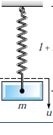
Consider the vibrating mass in Figure $1,$ then spring constant is $\beta^{2}$, there is no forcing function and damping force is $A \sin \omega t,$ the differential equation of motion:
$\Omega^{\prime \prime}(\tau)+\beta^{2} \Omega(\tau)=A \sin \omega t, \Omega(0)=\left(X_{0}-\alpha, \alpha-X_{0}\right)$,
$\Omega^{\prime}(0)=\left(V_{0}-\alpha, \alpha-V_{0}\right)$
Figure 1. Vibration of a spring
By fuzzy Elzaki transform method we have $E\left[\Omega^{\prime \prime}(\tau)\right]-\beta^{2} E[\Omega(\tau)]=A E[\sin \omega t]$.
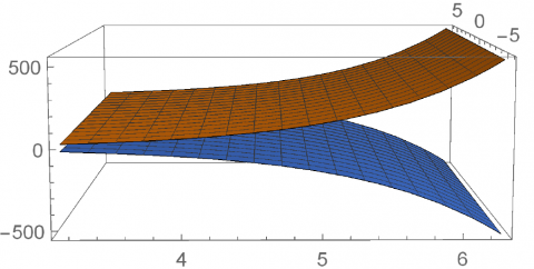
Case 1: If $\Omega(\tau)$ and $\Omega^{\prime}(\tau)$ are no. $2,$ then
$\begin{aligned} e[\underline{\Omega}(\tau)]=&\left(X_{0}-\alpha\right) \frac{u^{2}}{1+\beta^{2} u^{2}}+\left(V_{0}-\alpha\right) \frac{u^{3}}{1+\beta^{2} u^{2}}+\\ & \frac{A \omega}{\omega^{2}-\beta^{2}}\left[\frac{u^{3}}{1+\omega^{2} u^{2}}+\frac{u^{2}}{1+\beta^{2} u^{2}}\right] \end{aligned}$
$\begin{aligned} E[\underline{\Omega}(\tau)] &=\left(X_{0}-\alpha\right) \cos \beta t+\frac{\left(V_{0}-\alpha\right)}{\beta} \sin \beta t+\\ & \frac{A}{\omega^{2}-\beta^{2}}\left(\sin \omega t-\frac{\omega}{\beta} \sin \beta t\right) \end{aligned}$
$e[\bar{\Omega}(\tau)]=\left(\alpha-X_{0}\right) \frac{u^{2}}{1+\beta^{2} u^{2}}+\left(\alpha-V_{0}\right) \frac{u^{3}}{1+\beta^{2} u^{2}}+$
$\frac{A \omega}{\omega^{2}-\beta^{2}}\left[\frac{u^{3}}{1+\omega^{2} u^{2}}+\frac{u^{2}}{1+\beta^{2} u^{2}}\right]$
$E[\bar{\Omega}(\tau)]=\left(\alpha-X_{0}\right) \cos \beta t+\frac{\left(\alpha-V_{0}\right)}{\beta} \sin \beta t+$
$\frac{A}{\omega^{2}-\beta^{2}}\left(\sin \omega t-\frac{\omega}{\beta} \sin \beta t\right)$
Figure 2 shows the graph of this case.
Case 2: if $\Omega(\tau)$ is no. 1 and $\Omega^{\prime}(\tau)$ is no.2, then
$\begin{aligned} e[\underline{\Omega}(\tau)]=&\left(X_{0}-\alpha\right) \frac{u^{2}}{1-\beta^{2} u^{2}}-\left(V_{0}-\alpha\right) \frac{u^{3}}{1-\beta^{2} u^{2}}+\\ & \frac{A \omega}{\omega^{2}-\beta^{2}}\left[\frac{u^{3}}{1+\omega^{2} u^{2}}+\frac{u^{2}}{1+\beta^{2} u^{2}}\right] \end{aligned}$
$\begin{aligned} E[\underline{\Omega}(\tau)]=&\left(X_{0}-\alpha\right) \cosh \beta t-\frac{\left(V_{0}-\alpha\right)}{\beta} \sinh \beta t+\\ & \frac{A}{\omega^{2}-\beta^{2}}\left(\sin \omega t-\frac{\omega}{\beta} \sin \beta t\right) \end{aligned}$
$\begin{aligned} e[\bar{\Omega}(\tau)]=&\left(\alpha-X_{0}\right) \frac{u^{2}}{1-\beta^{2} u^{2}}-\left(\alpha-V_{0}\right) \frac{u^{3}}{1-\beta^{2} u^{2}}+\\ & \frac{A \omega}{\omega^{2}-\beta^{2}}\left[\frac{u^{3}}{1+\omega^{2} u^{2}}+\frac{u^{2}}{1+\beta^{2} u^{2}}\right] \end{aligned}$
$\begin{aligned} E[\bar{\Omega}(\tau)]=\left(\alpha-X_{0}\right) \cosh \beta t-\frac{\left(\alpha-V_{0}\right)}{\beta} \sinh \beta t+ & \frac{A}{\omega^{2}-\beta^{2}}\left(\sin \omega t-\frac{\omega}{\beta} \sin \beta t\right) \end{aligned}$
Figure 3 shows the graph of this case.
Figure 2. Case (1)
Figure 3. Case (2)
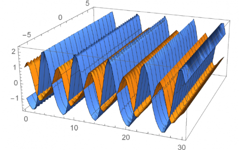
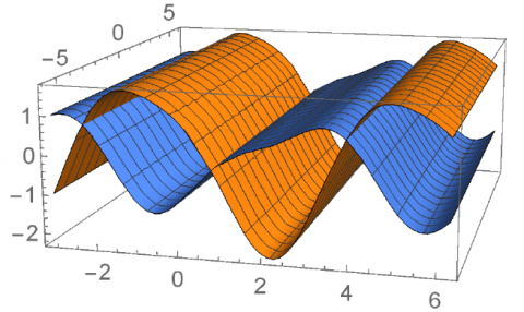
Case 3 : if $\Omega^{\prime}(\tau)$ be no. 1 and $\Omega(\tau)$ is no. 2 , then
$e[\underline \Omega(\tau)]=\left(X_{0}-\alpha\right) \frac{u^{2}}{1-\beta^{2} u^{2}}+\left(V_{0}-\alpha\right) \frac{u^{3}}{1-\beta^{2} u^{2}}+$$\frac{A \omega}{\omega^{2}-\beta^{2}}\left[\frac{u^{3}}{1+\omega^{2} u^{2}}+\frac{u^{2}}{1+\beta^{2} u^{2}}\right]$
$E[\underline\Omega(\tau)]=\left(X_{0}-\alpha\right) \cosh \beta t+\frac{\left(V_{0}-\alpha\right)}{\beta} \sinh \beta t+$$\frac{A}{\omega^{2}-\beta^{2}}\left(\sin \omega t-\frac{\omega}{\beta} \sin \beta t\right)$
$\begin{aligned} e[\bar{\Omega}(\tau)]=\left(\alpha-X_{0}\right) \frac{u^{2}}{1-\beta^{2} u^{2}}+\left(\alpha-V_{0}\right) \frac{u^{3}}{1-\beta^{2} u^{2}}+ & \frac{A \omega}{\omega^{2}-\beta^{2}}\left[\frac{u^{3}}{1+\omega^{2} u^{2}}+\frac{u^{2}}{1+\beta^{2} u^{2}}\right] \end{aligned}$
$\begin{aligned} E[\bar{\Omega}(\tau)]=\left(\alpha-X_{0}\right) \cosh \beta t+\frac{\left(\alpha-V_{0}\right)}{\beta} \sinh \beta t+& \frac{A}{\omega^{2}-\beta^{2}}\left(\sin \omega t-\frac{\omega}{\beta} \sin \beta t\right) \end{aligned}$
Figure 4 shows the graph of this case.
Case 4: If $\Omega(\tau)$ and $\Omega^{\prime}(\tau)$ are no. $1,$ then
$\begin{aligned} e[\underline\Omega(\tau)]=\left(X_{0}-\alpha\right) \frac{u^{2}}{1+\beta^{2} u^{2}}-\left(V_{0}-\alpha\right) \frac{u^{3}}{1+\beta^{2} u^{2}}+ & \frac{A \omega}{\omega^{2}-\beta^{2}}\left[\frac{u^{3}}{1+\omega^{2} u^{2}}+\frac{u^{2}}{1+\beta^{2} u^{2}}\right] \end{aligned}$
$\begin{aligned} E[\underline\Omega(\tau)] &=\left(X_{0}-\alpha\right) \cos \beta t-\frac{\left(V_{0}-\alpha\right)}{\beta} \sin \beta t+\\ & \frac{A}{\omega^{2}-\beta^{2}}\left(\sin \omega t-\frac{\omega}{\beta} \sin \beta t\right) \end{aligned}$
$\begin{aligned} e[\bar{\Omega}(\tau)]=&\left(\alpha-X_{0}\right) \frac{u^{2}}{1+\beta^{2} u^{2}}-\left(\alpha-V_{0}\right) \frac{u^{3}}{1+\beta^{2} u^{2}}+\\ & \frac{A \omega}{\omega^{2}-\beta^{2}}\left[\frac{u^{3}}{1+\omega^{2} u^{2}}+\frac{u^{2}}{1+\beta^{2} u^{2}}\right] \end{aligned}$
$\begin{aligned} E[\bar{\Omega}(\tau)] &=\left(\alpha-X_{0}\right) \cos \beta t-\frac{\left(\alpha-V_{0}\right)}{\beta} \sin \beta t+\\ & \frac{A}{\omega^{2}-\beta^{2}}\left(\sin \omega t-\frac{\omega}{\beta} \sin \beta t\right) \end{aligned}$
Figure 5 shows the graph of this case.
Figure 4. Case (3)
Figure 5. Case (4)
The solution of an initial value problem addresses several physical problems. The procedure demonstrates that many physical problems that have the same mathematical model in addition to a fundamental relationship between physics and mathematics. There are many different forces acting upon the mass on a spring, the force is positive if it acts in the downward direction whereas the force will be negative if it acts in the upward direction. Therefore, this paper considered the mass motion of the spring in a few specifics as the first step in the investigation of more complex vibrational systems is the understanding of the behavior of this basic mechanism.
|
O.N |
odd number |
|
E.N |
Even number |
|
no.1 |
(i)-differentiable |
|
no.2 |
(ii)-differentiabl |
|
E |
Elzaki transform |
|
S |
Sumudu transform |
|
Greek symbols |
|
|
$\oplus$ |
fuzzy addition |
|
$\ominus$ |
fuzzy Subtraction |
|
$\beta^{2}$ |
spring constant |
|
$A \sin \omega t$ |
damping force |
[1] Clark, B.L. (2017). Ode to Applied Physics: The Intellectual Pathway of Differential Equations in Mathematics and Physics Courses: Existing Curriculum and Effective Instructional Strategies.
[2] Eslaminasab, M., Abbasbandy, S. (2015). Study on usage of Elzaki transform for the ordinary differential equations with non-constant coefficients. International Journal of Industrial Mathematics, 7(3): 277-281.
[3] Friedman, M., Ma, M., Kandel, A. (1999). Numerical solutions of fuzzy differential and integral equations. Fuzzy Sets and Systems, 106(1): 35-48. https://doi.org/10.1016/S0165-0114(98)00355-8
[4] Arshad, S., Lupulescu, V. (2011). On the fractional differential equations with uncertainty. Nonlinear Analysis: Theory, Methods & Applications, 74(11): 3685-3693. https://doi.org/10.1016/j.na.2011.02.048
[5] ElJaoui, E., Melliani, S., Chadli, L.S. (2015). Solving second-order fuzzy differential equations by the fuzzy Laplace transform method. Advances in Difference Equations, (1): 1-14. https://doi.org/10.1186/s13662-015-0414-x
[6] Patel, K.R., Desai, N.B. (2017). Solution of fuzzy initial value problems by fuzzy Laplace transform. Kalpa Publications in Computing, 2: 25-37.
[7] Çitil, H.G. (2019). Investigation of a fuzzy problem by the fuzzy Laplace transform. Applied Mathematics and Nonlinear Sciences, 4(2): 407-416. https://doi.org/10.2478/AMNS.2019.2.00039
[8] Haydar, A.K., Hassan, R.H. (2016). Generalization of fuzzy laplace transforms of fuzzy fractional derivatives about the general fractional order n-1<β<n. Mathematical Problems in Engineering. https://doi.org/10.1155/2016/6380978
[9] Bagyalakshmi, M., SaiSundarakrishnan, G. (2020). Tarig projected differential transform method to solve fractional nonlinear partial differential equations. Boletim da Sociedade Paranaense de Matemática, 38(3): 23-46. https://doi.org/10.5269/bspm.v38i3.34432
[10] Rahman, N.A.A., Ahmad, M.Z. (2018). Fuzzy Sumudu transform for solving system of linear fuzzy differential equations with fuzzy constant coefficients. Preprints 2018. https://doi.org/10.20944/preprints201806.0121.v1
[11] Rahman, N.A.A., Ahmad, M.Z. (2015). Applications of the fuzzy Sumudu transform for the solution of first order fuzzy differential equations. Entropy, 17(7): 4582-4601. https://doi.org/10.3390/e17074582
[12] Štěpnička, M., Lehmke, S. (2005). Approximation of Fuzzy Functions by Extended Fuzzy Transforms. Reusch B. (eds) Computational Intelligence, Theory and Applications. Advances in Soft Computing, vol 33. Springer, Berlin. https://doi.org/10.1007/3-540-31182-3_16
[13] Bulut, H., Baskonus, H.M., Belgacem, F.B.M. (2013). The analytical solution of some fractional ordinary differential equations by the Sumudu transform method. In Abstract and Applied Analysis. https://doi.org/10.1155/2013/203875
[14] Yang, C., Hou, J. (2013). Numerical solution of integro-differential equations of fractional order by Laplace decomposition method. Wseas Transactions on Mathematics, 12(12): 1173-1183. https://doi.org/10.1007/BF01935570
[15] Mohammed, D.S. (2014). Numerical solution of fractional integro-differential equations by least squares method and shifted Chebyshev polynomial. Mathematical Problems in Engineering. https://doi.org/10.1155/2014/431965
[16] Jena, R.M., Chakraverty, S. (2019). Solving time-fractional Navier–Stokes equations using homotopy perturbation Elzaki transform. SN Applied Sciences, 1(1): 16. https://doi.org/10.1007/s42452-018-0016-9
[17] Verma, D., Alam, A. (2020). Analysis of simultaneous differential equations by elzaki transform approach. Science, Technology and Development Journal, 9(1): 364-367.
[18] Lu, D., Suleman, M., He, J.H., Farooq, U., Noeiaghdam, S., Chandio, F.A. (2018). Elzaki projected differential transform method for fractional order system of linear and nonlinear fractional partial differential equation. Fractals, 26(3): 1850041. https://doi.org/10.1142/S0218348X1850041X
[19] Ziane, D., Elzaki, T.M., Cherif, M.H. (2018). Elzaki transform combined with variational iteration method for partial differential equations of fractional order. Fundamental Journal of Mathematics and Applications, 1(1): 102-108. https://doi.org/10.33401/fujma.415892
[20] Singh, P., Sharma, D. (2019). Comparative study of homotopy perturbation transformation with homotopy perturbation Elzaki transform method for solving nonlinear fractional PDE. Nonlinear Engineering, 9(1): 60-71. https://doi.org/10.1515/nleng-2018-0136
[21] Ige, O.E., Oderinu, R.A., Elzaki, T.M. (2019). Adomian polynomial and elzaki transform method for solving Klein Gordon equations. International Journal of Applied Mathematics, 32(3): 451. https://doi.org/10.12732/ijam.v32i3.7
[22] Khalouta, A., Kadem, A. (2018). Mixed of Elzaki transform and projected differential transform method for a nonlinear wave-like equations with variable coefficients. Preprints 2018. https://doi.org/10.20944/preprints201808.0088.v1
[23] Elzaki, T.M. (2011). On the Elzaki transforms and system of partial diffrential equations. Advances in Theoretical and Applid Mathematics, 1: 115-123.
[24] Elzaki, T.M. (2011). The new integral transform ‘Elzaki transform’. Global Journal of Pure and Applied Mathematics, 7(1): 57-64.
[25] Adam, B.A. (2015). A comparative study of Adomain decomposition method and the new integral transform “Elzaki Transform”. International Journal of Applied Mathematical Research, 4(1): 8-14. https://doi.org/10.14419/ijamr.v4i1.3799
[26] Khalid, M., Sultana, M., Zaidi, F., Arshad, U. (2015). Application of Elzaki transform method on some fractional differential equations. Mathematical Theory and Modeling, 5(1): 89-96.
[27] Bede, B., Gal, S.G. (2005). Generalizations of the differentiability of fuzzy-number-valued functions with applications to fuzzy differential equations. Fuzzy Sets and Systems, 151(3): 581-599. https://doi.org/10.1016/j.fss.2004.08.001
[28] Hooshangian, L., Allahviranloo, T. (2014). A new method to find fuzzy nth order derivation and applications to fuzzy nth order arithmetic based on generalized h-derivation. An International Journal of Optimization and Control: Theories & Applications (IJOCTA), 4(2): 105-121. https://doi.org/10.11121/ijocta.01.2014.00183
[29] Chalco-Cano, Y., Roman-Flores, H. (2008). On new solutions of fuzzy differential equations. Chaos, Solitons & Fractals, 38(1): 112-119. https://doi.org/10.1016/j.chaos.2006.10.043
[30] Allahviranloo, T., Ahmady, E., Ahmady, N. (2009). A method for solving n th order fuzzy linear differential equations. International Journal of Computer Mathematics, 86(4): 730-742. https://doi.org/10.1080/00207160701704564
[31] Haydar, A.K. (2015). Fuzzy Sumudu transform for fuzzy nth-order derivative and solving fuzzy ordinary differential equations. International Journal of Science and Research, 4: 1372-1378.
[32] Jafari, R., Razvarz, S. (2018). Solution of fuzzy differential equations using fuzzy Sumudu transforms. Mathematical and Computational Applications, 23(1): 5. https://doi.org/10.3390/mca23010005