Nicola Germano* | Camilla Lops | Sergio Montelpare | Guido Camata | Renato Ricci
© 2020 IIETA. This article is published by IIETA and is licensed under the CC BY 4.0 license (http://creativecommons.org/licenses/by/4.0/).
OPEN ACCESS
The present paper aims to expose the Mesoscale-Microscale numerical approach adopted for studying the air fluxes inside an urban area located in the city of Pescara (Italy). The data, recorded by a real anemometer, are compared with three Mesoscale models (Pleim-Xiu, Blackadar and MRF-LSM), each of them presents five nested domains. On the bases of the monthly values of Root Mean Square Error, BIAS and Standard Deviation, the most accurate mesoscale model is identified and evaluated. On the Microscale side, instead, two cylindrical domains are studied. The first model considers only the topography of the terrain, whereas the other also adds the buildings present inside the investigated area. The domains, with a diameter of 6 [km] and a height equal to 0.5 [km], are studied by assuming the incoming wind from four different directions. Comparisons are then made among wind speeds and directional inflows obtained from the two models. Mesoscale analyses are carried out with the weather forecast software MM5, and Microscale simulations are performed with the commercial software STAR-CCM+.
urban physics, multiscale approach, macroscale analysis, microscale analysis, MM5, CFD
The well-known problem of rising temperatures inside cities is a phenomenon related to climate change effects as experienced in recent years. The analysis conducted by the World Meteorological Organization (WMO) [1] underlines how the concentration of greenhouse gases reached record levels in 2018 with carbon dioxide (CO2) even 147% higher than pre-industrial levels. The last five years have been the hottest in the decade 2010-2019 with temperatures almost 1 [°C] more elevated than the average recorded in the 20th century.
By focusing on the study of the urban fabric, it is easy to imagine how these conditions play a fundamental role in people health. Among the adverse effects, Urban Heat Islands (UHI) play an essential role. In fact, in 2018 UHIs exposed to heatwaves 220 million people over 65 years of age [1].
One method that is increasingly being used to try to mitigate some of these effects is Computational Fluid Dynamics (CFD) analysis. Various works proved the effectiveness of this typology of simulations for studying the urban fabric in different sectors. Toparlar et al. [2] identified 37 different categories in which these analyses have been used. Toparlar et al. [3] conducted a study to predict urban temperatures in the Bergpolder Zuid region of Rotterdam (Netherlands); Miao et al. [4], coupling a weather forecast model with CFD, studied the air flow and dispersion of pollutants in a complex urban area of Beijing (China); Montelpare et al. [5], instead, provided a Mesoscale-Microscale numerical approach able to select the best orientation of the buildings according to the local wind in the city of Ancona (Italy).
In this study, two buildings were also selected to carry out energy analyses.
The present work intends to provide the fundamental study of a coupling process which, among other things, can be an essential tool for studying wind flows within advanced energy analyses.
This article is structured as follows: the adopted methodology is briefly described in Section 2. In particular, the Mesoscale approach is presented in Section 2.1 where the meteorological model (Section 2.1.1), the numerical set-up (Section 2.1.2) and the obtained results (Section 2.1.3) are shown. The Microscale method is, then, described in Section 2.2 with the computational model (Section 2.2.1), the boundary conditions (Section 2.2.2) and the findings coming from the performed simulations (Section 2.2.3). Finally, Section 3 draws the main conclusions.
In the present work, an urban area is studied by means of Mesoscale and Microscale analyses. Within the framework, further simulations are referred to the Microscale model. The combination of these two analyses will provide more accurate data for better quality energy studies.
2.1 Mesoscale approach
To describe the climatology of the area and to assess the wind inside the study area, Mesoscale analyses were carried out over a period of one year (from 1st July 2016 to 30th June 2017). The area in question is located in the town of Pescara on the Italian Adriatic coast.
2.1.1 Meteorological model
The software developed by the Pennsylvania State University (PSU) and the National Center for Atmospheric Research (NCAR), Mesoscale Model Fifth Generation (MM5) [6], was selected to perform Macroscale analysis. MM5 is a limited-area, nonhydrostatic, terrain-following sigma-coordinate model designed to simulate or predict mesoscale atmospheric circulation.
2.1.2 The numerical set-up
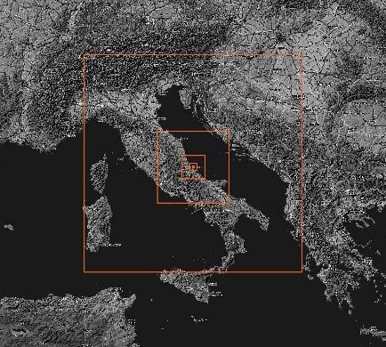
In order to take into account weather phenomena from the synoptic scale to the local one, the one-way nesting procedure was used on five nested domains (Figure 1). The characteristics of the considered domains are summarised in Table 1 All domains have the same centre (42°26'34'' northern latitude and 14°12'26'' eastern longitude) and number of grid points. The Arakawa-Lamb B-staggering scheme (Figure 2) is used, and a ratio of the increasing spatial dimension is equal to 3: 1.
Table 1. Macroscale domains
|
Domain |
Grid Spacing |
Grid Points |
Domain Extension |
|
D5 |
0.4 [km] |
31x31 |
12x12 [km2] |
|
D4 |
1.2 [km] |
31x31 |
36x36 [km2] |
|
D3 |
3.6 [km] |
31x31 |
108x108 [km2] |
|
D2 |
10.8 [km] |
31x31 |
324x324 [km2] |
|
D1 |
32.4 [km] |
31x31 |
972x972 [km2] |
Figure 1. Domain nesting
Figure 2. Arakawa B nesting schema
By analysing the largest domain (D1), it is possible to study phenomena that occur weekly or monthly. In contrast, with the smallest one (D5) it is possible to describe better local convective phenomena such as sea breezes or hill breezes that occur with a frequency of 12h or 24h [7].
The input meteorological data are the NCEP (National Centers for Environmental Prediction) ds083.2 datasets which belong to FNL (Final Global Data Assimilation System) category. These data are available from 1999 to current days, and they have a grid resolution of 1° x 1° with a 6 hours time interval (00:00, 06:00, 12:00, 18:00 UTC).
The simulating features of the MM5 surface meteorological parameters are evaluated by using three different combinations of the planetary boundary layer (PBL) and land surface model (LSM) parameterisation schemes. The first one corresponds to the PBL of Medium-Range Forecast model (MRF) developed by Hong and Pan [8] coupled with the NOAH LSM. The second combination comprises the PBL developed by Pleim and Chang [9] coupled with the LSM developed by Pleim and Xiu [10]. The third and last model here evaluated is the one created by Blackadar [11].
2.1.3 Macroscale results
In order to compare the results obtained from the MM5 analysis with the data collected from a real anemometer, the outputs are converted from a 4 minutes time step to a 10 minutes time step. The real anemometer, located at the “G. d’Annunzio” University of Pescara (42°27’07” northern latitude and 14°13’29” eastern longitude), belongs to a private and professional network of urban weather stations in Italy, developed in 2010. More than 50 weather stations in various cities are part of this network.
For each of the three models (MRF-LSM, Pleim-Xiu and Blackadar) the values of pressure, humidity, temperature, wind speed and direction at five different altitudes were studied: 10 [m], 30 [m], 71 [m], 122 [m] and 204 [m]. Then, monthly values of Root Mean Square Error (RMSE), BIAS and Standard Deviation (SD) were calculated.
These three parameters showed that the MRF-LSM model, in accordance with Germano et al. [12], is the most accurate if the outputs are compared with the data obtained from the real anemometer.
The Blackadar model, instead, predicts values that are the most deviate from the real data taking into account the wind pressure and speed; considering the temperature and wind direction, the Pleim-Xiu model shows a more significant deviation from the measured data.
2.2 Microscale approach
Microscale simulations were performed in STAR-CCM+ commercial software, and two different numerical models were elaborated. In the first case, the only topography of the terrain was modelled, whereas, in the other, the buildings present in the area were also considered. This type of study allows estimating the alterations of the direction and intensity of the wind within the urban area due to the presence of buildings.
2.2.1 Computational domain
The computational domain used for this study is a cylinder having the same centre of the domains of the Mesoscala (42°26’34’’ northern latitude and 14°12’26’’ eastern longitude). The domain presents two different zones: the outer layer with a diameter of 6 [km] characterised by a coarse mesh, and the inner circle with a diameter of 3 [km] where a thicker mesh is generated. The buildings are located in the inner area with a diameter of 1 [km].
The lateral surface was divided into 12 circular sectors every 30° to take into account different incoming wind directions. In this research, 4 main directions corresponding to the 4 cardinal points were studied.
The total diameter of the domain, therefore, is 6 [km] and a total height of 0.5 [km] was chosen in order to have a blockage ratio less than 3% as suggested by Blocken [13].
Buildings were modelled with their real shape and size thanks to the information contained in the regional cartography (CTR) as well as the topography of the terrain, elaborated from the discretisation of the isocontour.
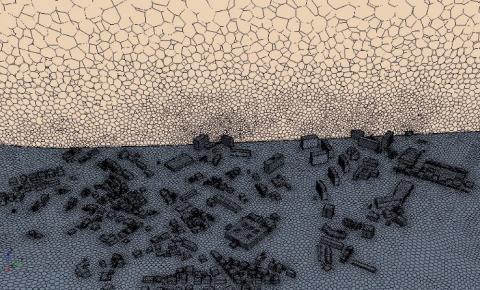
Triangular and polyhedral elements were adopted, respectively, for the surface and volume mesh. Prismatic elements were also inserted near the ground and buildings (when present). The mesh was set to be more accurate around the terrain and buildings, by inserting smaller elements, and less precise far away from them (Figure 3). Table 2 summarizes the number of elements obtained for each of the two models.
Figure 3. Mesh detail
Table 2. Domain elements
|
Model |
Faces |
Edges |
Cells |
Vertices |
|
Terrain |
359,694 |
1,513 |
1,697,157 |
8,514,821 |
|
Terrain Buildings |
491,214 |
33,862 |
2,645,737 |
12,212,485 |
2.2.2 Boundary conditions
Depending on the analysed wind direction, the side sectors was set with a boundary condition (BC) of the flow corresponding to Velocity Inlet or Pressure Outlet. For each considered directions, six sectors were specified as Velocity Inlet and the other six as Pressure Outlet. The surface of the land and buildings was modelled as Wall, while the top surface of the domain was set as Symmetry Plane.
At BC inlet, a logarithmic wind speed profile was adopted (Eq. (1)) by setting z0=0.05 [m] and a reference wind speed of 6.0 [m/s]. For each of the four simulations the parameter q was changed in order to consider the different direction of the incoming wind.
The unsteady Reynolds-Averaged Navier-Stokes (U-RANS) model was selected for numerical simulations and the turbulence was considered by means of the two-equation k-ε model, in which transport equations are solved for the turbulent kinetic energy k [m2/s2] and turbulence dissipation rate ε [m2/s3] provided by Richards and Hoxey [14].
$U(z)=\frac{u^{*}}{k} \ln \left(\frac{Z+z_{0}}{z_{0}}\right)$ (1)
$k=\frac{u^{*^{2}}}{\sqrt{C_{\mu}}}$ (2)
$\varepsilon(z)=\frac{u^{*^{3}}}{k\left(z+z_{0}\right)}$ (3)
where, k is 0.42, u* [m/s] is the friction velocity of the atmospheric boundary layer, C is 0.09 (is a constant), z0 [m] is the length of the aerodynamic roughness and z [m] is the height coordinate.
2.2.3 Microscale results
For the sake of the brevity, the only results obtained from the analysis with the incoming wind from the North are here presented.
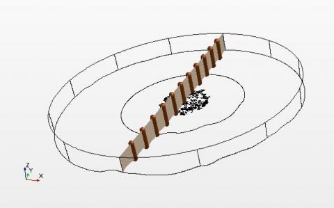
The data were extracted by discretising every 500 [m] the YZ plane passing through the centre of the domain (Figure 4). For each position, the wind speed and the directional inflows concerning the elevation were graphed.
Figure 4. Extraction points
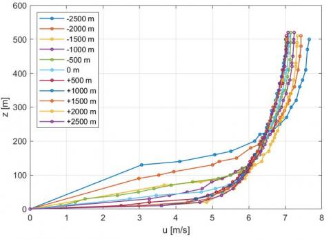
Analyzing the wind speed graphs between the model without buildings (Figure 5) and with the buildings (Figure 6) the data extracted from y=2500 [m] to y=1000 [m] show a substantially similar trend since it is the part of the domain not yet affected by buildings. From y=500 [m] onwards, however, there is a different trend with a decrease of the wind due to the impact that the air flux has on the first buildings encountered along the way. At higher levels the results obtained by the two models (with and without buildings) may be overlapped because they have similar values.
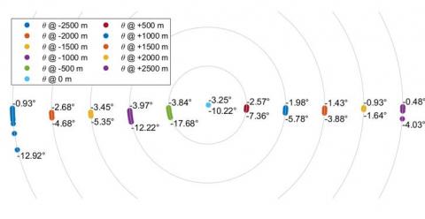
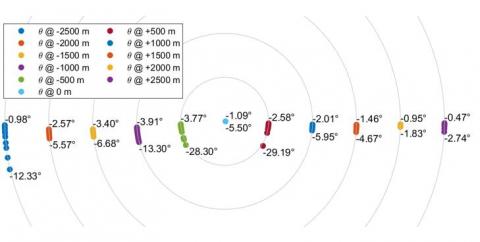
Even analyzing the results of the directional inflows (Figure 7 and Figure 8), it is possible to notice that there is an evident difference in proximity of the buildings, i.e. between y=500 [m] and y=-500 [m]. Away from the buildings, the differences between the two models are less noticeable.
Figure 5. Wind speed - model without buildings
Figure 6. Wind speed - model with buildings
Figure 7. Relative directional inflow - model without buildings
Figure 8. Relative directional inflow - model with buildings
The purpose of this work was to evaluate the use of Mesoscale and Microscale analyses for the definition of a coupling procedure, capable of providing more accurate data for advanced energy simulations. Better quality values, in fact, become crucial in case of advanced technological systems such as buildings with ventilated façades, for which information about incoming wind flows obtained from the Mesoscale are extremely useful.
The research was divided into two parts: in the first part, Mesoscale analyses were carried out, whereas the second part is dedicated to Microscale analyses. Mesoscale analyses, performed with the MM5 software, underlined that the MRF-LSM model, unlike the Blackadar and Pleim-Xiu models, is the most accurate for the investigated area. The MRF-LSM estimated values showed better agreement with the data measured by a real anemometer.
Microscale analyses, on the other hand, were performed for estimating the impact of buildings on wind intensity and direction inside an urban area. Two models and four incoming wind directions were analysed. The first model was elaborated considering only the topography of the terrain. The presence of buildings was, instead, taken into account in the second model. The obtained results underline how the building located in the area can drastically affect wind speed and direction. In fact, a decrease and deviation of the speed near the buildings are predicted.
|
BC |
Boundary Condition |
|
BES |
Building Energy Simulations |
|
CFD |
Computational Fluid Dynamic |
|
CTR |
Carta Tecnica Regionale (in the Italian wording) |
|
FNL |
Final Global Data Assimilation System |
|
LSM |
Land Surface Model |
|
MM5 |
Mesoscale Model Fifth Generation |
|
MRF |
Medium-Range Forecast model |
|
NCAR |
National Center for Atmospheric Research |
|
NCEP |
National Centers for Environmental Prediction |
|
PBL |
Planetary Boundary Layer |
|
PSU |
Pennsylvania State University |
|
RMSE |
Root Mean Square Error |
|
SD |
Standard Deviation |
|
UHI |
Urban Heat Island |
|
U-RANS |
Unsteady Reynolds-Averaged Navier |
|
UTC |
Coordinated Universal Time |
|
WMO |
World Meteorological Organization |
[1] WMO Provisional Statement on the State of the Global Climate in 2019. https://public.wmo.int/en/resources/library/wmo-provisional-statement-state-of-global-climate-2019, accessed on Nov. 23, 2020.
[2] Toparlar, Y., Blocken, B., Maiheu, B., van Heijst, G.J.F. (2017). A review on the CFD analysis of urban microclimate. Renewable and Sustainable Energy Reviews, 80: 1613-1640. https://doi.org/10.1016/j.rser.2017.05.248
[3] Toparlar, Y., Blocken, B., Vos, P., van Heijst, G.J.F., Janssen, W.D., van Hooff, T., Montazeri, H., Timmermans, H.J.P. (2015). CFD simulation and validation of urban microclimate: A case study for Bergpolder Zuid, Rotterdam. Building and Environment, 83: 79-90. https://doi.org/10.1016/j.buildenv.2014.08.004
[4] Miao, Y., Liu, S., Chen, B., Zhang, B., Wang, S., Li, S. (2013). Simulating urban flow and dispersion in Beijing by coupling a CFD model with the WRF model. Advances in Atmospheric Sciences, 30(6): 1663-1678. https://doi.org/10.1007/s00376-013-2234-9
[5] Montelpare, S., D’Alessandro, V., Lops, C., Costanzo, E., Ricci, R. (2019). A Mesoscale-Microscale approach for the energy analysis of buildings. Journal of Physics: Conference Series, 1224(1). https://doi.org/10.1088/1742-6596/1224/1/012022
[6] Grell, G.A., Dudhia, J., Stauffer, D. (1994). A description of the fifth-generation Penn State/NCAR Mesoscale Model (MM5) (No. NCAR/TN-398+STR). University Corporation for Atmospheric Research. https://doi.org/10.5065/D60Z716B
[7] Burton, T., Sharpe, D., Jenkins, N., Bossanyi, E. (2001). Wind Energy Handbook. John Wiley & Sons, Ltd. http://dx.doi.org/10.1002/0470846062
[8] Hong, S., Pan, H. (1996). Nonlocal boundary layer vertical diffusion in a medium- range forecast model. Monthly Weather Review, 124: 2322-2339. https://doi.org/10.1175/1520-0493%281996%29124%3C2322:NBLVDI%3E2.0.CO;2
[9] Pleim, J.E., Chang, J.S. (1992). A non-local closure model for vertical mixing in the convective boundary layer. Atmospheric Environment. Part A. General Topics, 26(6): 965-981. http://dx.doi.org/10.1016/0960-1686%2892%2990028-J
[10] Xiu, A.J., Pleim, J.E. (2001). Development of a land surface model. Part I: Application in a mesoscale meteorological model. Journal of Applied Meteorology and Climatology, 40(2): 192-209. http://dx.doi.org/10.1175/1520-0450%282001%29040%3C0192:DOALSM%3E2.0.CO;2
[11] Blackadar, A.K. (1976). Modeling the nocturnal boundary layer. In: Proceedings of the Third Symposium on Atmospheric Turbulence, Diffusion, and Air Quality, American Meteorological Society, Rayeligh, pp. 46-49.
[12] Germano, N., Lops, C., Matera, S., Montelpare, S., Camata, G. (2020). A multiscale approach for creating boundary conditions for building energy analysis. TECNICA ITALIANA-Italian Journal of Engineering Science, 64(2-4): 298-302. https://doi.org/10.18280/ti-ijes.642-426
[13] Blocken, B. (2015). Computational fluid dynamics for urban physics: Importance, scales, possibilities, limitations and ten tips and tricks towards accurate and reliable simulations. Building Environment, 91: 219-245. https://doi.org/10.1016/j.buildenv.2015.02.015
[14] Richards, P.J., Hoxey, R.P. (1993). Appropriate boundary conditions for computational wind engineering models using the k-ϵ turbulence model. Journal of Wind Engineering and Industrial Aerodynamics, 46-47: 145-153. https://doi.org/10.1016/0167-6105%2893%2990124-7