Bikash C. Parida* | Bharat K. Swain | Nityananda Senapati | Srustisoumya Sahoo
© 2020 IIETA. This article is published by IIETA and is licensed under the CC BY 4.0 license (http://creativecommons.org/licenses/by/4.0/).
OPEN ACCESS
The current paper illustrates the consequence of viscous dissipation on the unsteady MHD flow of an incompressible viscous fluid over a vertical permeable surface embedded in a porous medium. The roles of chemical reaction and thermal radiation has made the study more interesting. The Perturbation method has been applied to solve the coupled and nonlinear governing equations. It is found that the present solutions are in very good agreement with the previous solutions. The important findings are: increasing values of Eckert number (Ec) enhances the velocity of the fluid flow. The viscous dissipation convincingly increases the temperature. This analysis is of great interest in many applications such as polymer processing flows, condensation process of metallic plate in cooling bath, aerodynamic extrusion of plastic sheets etc.
chemical reaction, MHD, nusselt number, porous medium, sherwood number, skin friction, thermal radiation, viscous dissipation
Magnetohydrodynamics (MHD) presents the magnetic properties of electrically conducting fluid such as plasma, liquid metals, salt water etc. These fluids also exhibit the viscosity property which is responsible for the flow of fluid. It takes energy from the motion of fluid and transfer it into internal energy. As a result, the fluid gets heated. This dissipation process has applications in polymer processing flows, aerodynamic heating in the thin boundary layer around high speed aircraft etc. Many researchers have studied the significant effects of viscous dissipation on MHD flow. Devi et al. [1] investigated the effect of viscous and joule dissipation on MHD flow past a stretching porous surface. Murugesan and Kumar [2], Kumari and Goyal [3], Kumar and Reddy [4] and Rani et al. [5] have considered the viscous dissipation effects under distinct flow domain.
Now-a-days, it is also of great interest to study thermal radiation and chemical reaction in MHD flow of the fluid. Fluid temperature greater than absolute zero emits thermal radiation. When the fluid flows it results in change acceleration a dipole oscillation which produces electro-magnetic radiation. Mass transfer with chemical reaction also acts a vital role in the fluid flow. Many authors ([6-12]) tried to study the influences of thermal radiation and chemical reaction on MHD flow along with viscous dissipation. They solved the governing equations either analytically or numerically.
Further, the roles of external magnetic field and porous medium in MHD heat transfer flow are very much of industrial importance. These types of engineering problems are very relevant in geothermal, energy extractions, oil exploration and the boundary layer control in the field of aerodynamics. Therefore, many investigations have been accomplished by the renowned authors. Makinde et al. [13-15] elucidated numerically the MHD fluid flows past a vertical plate as well as past a slippery stretching. In all of their study, they considered the flow system in a porous medium. Swain and Senapati [16] examined the mass transfer effect on MHD free convective flow embedded in a porous medium. Uddin [17] also carried out his research in a Porous Medium.
The objective of the present study is to analyze viscous dissipation effect on an unsteady MHD free convective flow embedded in a porous medium. Viscous dissipation effect was not attained by Prakash et al. [6], but here we consider it. The expressions for velocity, skin friction, Sherwood number, Nusselt number are obtained using the perturbation technique. These are compared with the previous results for different physical parameters. The present results agree well with the previous results. Moreover, the works of Prakash et al. [6] and Kim [18] have been discussed as special cases. The significance of the physical parameters also studied graphically. Here, all the calculations and graphs are carried out using MATLAB software.
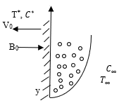
The geometrical flow of the problem is shown in Figure 1. A two-dimensional boundary layer flow of a viscous incompressible fluid past a semi-infinite vertical permeable plate placed in a uniform porous medium is observed. The fluid is also assumed to be electrically conducting and heat absorbing. An external magnetic field B0 is applied in the presence of thermal and concentration buoyancy effects. The Hall and ion slip effects are considered negligible. External electric field is assumed to be zero and the electric field due to the polarization of charges is negligible. The plate is maintained at constant temperature Tw and concentration Cw. which is higher than the ambient temperature T∞ and concentration C∞, respectively. Since we have taken semi-infinite plane surface, the flow variables are the functions of y* and t* only. Under these assumptions, the governing equations are given by;
$\frac{\partial v^{*}}{\partial y^{*}}=0$, (1)
$\frac{\partial u^{*}}{\partial t^{*}}+v^{*} \frac{\partial u^{*}}{\partial y^{*}}=-\frac{1}{\rho} \frac{\partial p^{*}}{\partial x^{*}}+v \frac{\partial^{2} u^{*}}{\partial y^{* 2}}-\frac{\sigma B_{0}^{2}}{\rho} u^{*}+$
$g \beta_{T}\left(T^{*}-T_{\infty}\right)+g \beta_{C}\left(C^{*}-C_{\infty}\right)-\frac{v}{K^{*}} u^{*}$, (2)
$\frac{\partial T^{*}}{\partial t^{*}}+v^{*} \frac{\partial T^{*}}{\partial y^{*}}=\frac{K}{\rho C_{p}} \frac{\partial^{2} T^{*}}{\partial y^{* 2}}-\frac{1}{\rho C_{p}} \frac{\partial q_{r}^{*}}{\partial y^{*}}-\frac{Q_{0}}{\rho C_{p}}\left(T^{*}-\right.$
$\left.T_{\infty}\right)+\frac{Q_{1}^{*}}{\rho C_{p}}\left(C^{*}-C_{\infty}\right)+\frac{D_{m}}{C_{s}} \frac{K_{T}}{\rho C_{p}} \frac{\partial^{2} C^{*}}{\partial y^{* 2}}+\frac{\mu}{\rho C_{p}}\left(\frac{\partial u^{*}}{\partial y^{*}}\right)^{2}$, (3)
$\frac{\partial C^{*}}{\partial t^{*}}+v^{*} \frac{\partial C^{*}}{\partial y^{*}}=D \frac{\partial^{2} C^{*}}{\partial y^{* 2}}-R\left(C^{*}-C_{\infty}\right)$. (4)
The radiative heat flux is taken, which has been given by Pal and Talukdar [19] and Cogley et al. [20] as:
$\frac{\partial q_{r}^{*}}{\partial y^{*}}=4\left(T^{*}-T_{\infty}\right) I^{\prime}$, (5)
where, $I^{\prime}=\int_{0}^{\infty} K_{w \lambda} \frac{\partial e_{b \lambda}}{\partial T^{*}} d \lambda, K_{w \lambda}$ is the absorption coefficient at the wall and $e_{b \lambda}$ is Planck's function.
Figure 1. Flow geometry
Under the assumption stated above, the initial and boundary conditions for the velocity distribution involving slip flow, temperature, and concentration distributions are defined as:
$u^{*}=u_{s l i p}^{*}=\frac{\sqrt{k}}{\alpha} \frac{\partial u^{*}}{\partial y^{*}}, T^{*}=T_{w}+\epsilon\left(T_{w}-T_{\infty}\right) e^{n^{*} t^{*}}$
$C^{*}=C_{w}+\epsilon\left(C_{w}-C_{\infty}\right) e^{n^{*} t^{*}}$ at $y^{*}=0$ (6)
$\begin{aligned} u^{*}=U_{\infty}^{*}=U_{0}\left(1+\epsilon e^{n^{*} t^{*}}\right), T^{*} & \rightarrow T_{\infty}, C^{*} \rightarrow \\ C_{\infty} \text { as } y^{*} \rightarrow \infty & \end{aligned}$ (7)
From Eq. (1) we know that the suction velocity near the plate surface is either a constant or a function of time only. Consequently, it is considered that
$v^{*}=-V_{0}\left(1+\epsilon A e^{n^{*} t^{*}}\right)$, (8)
where, V0 is the mean suction velocity and $\epsilon A \ll 1$. The negative sign indicates that the suction velocity is pointed towards the plate.
In the free stream Eq. (2) gives
$-\frac{1}{\rho} \frac{d p^{*}}{d x^{*}}=\frac{d U_{\infty}^{*}}{d t^{*}}+\frac{\sigma}{\rho} B_{0}^{2} U_{\infty}^{*}+\frac{v}{K^{*}} U_{\infty}^{*}$ (9)
The non- dimensional quantities used in the text are:
$u=\frac{u^{*}}{U_{0}}, \quad v=\frac{v^{*}}{V_{0}}, y=\frac{v_{0} y^{*}}{v}, U_{\infty}=\frac{U_{\infty}^{*}}{U_{0}}, t=\frac{V_{0}^{2} t^{*}}{v}, \theta=$$\frac{T^{*}-T_{\infty}}{T_{w}-T_{\infty}}$ (10)
$C=\frac{C^{*}-C_{\infty}}{C_{W}-C_{\infty}}, n=\frac{n^{*} v}{V_{0}^{2}}, G r=\frac{\rho g v\left(T_{w}-T_{\infty}\right) \beta_{T}}{U_{0} V_{0}^{2}}, M=$ $\frac{\sigma v B_{0}^{2}}{\rho V_{0}^{2}}, S c=\frac{v}{D}$
$Q_{1}=\frac{Q_{1}^{*} v\left(C_{w}-C_{\infty}\right)}{\rho C_{p} V_{o}^{2}\left(T_{w}-T_{\infty}\right)}, \gamma=\frac{R v}{V_{0}^{2}}, D u=\frac{D_{m} k_{T}\left(C_{w}-C_{\infty}\right)}{C_{S} K\left(T_{w}-T_{\infty}\right)}, K=$$\frac{V_{0}^{2} K^{*}}{v^{2}}$
$E c=\frac{V_{0}^{2}}{C p\left(T_{w}-T_{\infty}\right)}, G m=\frac{\rho g v\left(C_{w}-C_{\infty}\right) \beta_{C}}{U_{0} V_{0}^{2}}, P r=\frac{\mu C_{p}}{k}$
$\phi=\frac{Q_{0} v}{\rho C_{p} V_{o}^{2}}, F=\frac{4 v I^{\prime}}{\rho C_{p} V_{o}^{2}}$
Considering the above dimensionless variables, the Eq. (2) - (4) can be written in a dimensionless form as:
$\frac{\partial u}{\partial t}-\left(1+\epsilon A e^{n t}\right) \frac{\partial u}{\partial y}=\frac{d U_{\infty}}{d t}+M_{1}\left(U_{\infty}-U\right)+\frac{\partial^{2} u}{\partial y^{2}}+$$G r \theta+G m C$, (11)
$\frac{\partial \theta}{\partial t}-\left(1+\epsilon A e^{n t}\right) \frac{\partial \theta}{\partial y}=\frac{1}{\operatorname{Pr}} \frac{\partial^{2} \theta}{\partial y^{2}}-F \theta+Q_{1} C+\emptyset \theta+$$\frac{D u}{\operatorname{Pr}}\left(\frac{\partial^{2} C}{\partial y^{2}}\right)+E c\left(\frac{\partial u}{\partial y}\right)^{2}$, (12)
$\frac{\partial C}{\partial t}-\left(1+\epsilon A e^{n t}\right) \frac{\partial C}{\partial y}=\frac{1}{S c} \frac{\partial^{2} C}{\partial y^{2}}-\gamma C$. (13)
where, $M_{1}=M+\frac{1}{K}$, M and K represents the magnetic force intensity and porosity parameter.
The corresponding non-dimensional initial and boundary conditions are given by:
$u=u_{s l i p}=\emptyset_{1} \frac{\partial u}{\partial y}, \theta=1+\epsilon e^{n t}$$C=1+\epsilon e^{n t} \quad$ at $y=0$ (14)
$U \rightarrow U_{\infty}=\left(1+\epsilon e^{n t}\right), \theta \rightarrow 0, C \rightarrow 0 \quad$ as $y \rightarrow \infty$ (15)
where, $\emptyset_{1}=\frac{\sqrt{K}}{\alpha} \frac{V_{0}}{v}$ is the permeability parameter.
To solve the coupled non-linear partial differential Eqns. (11)-(13) subject to the boundary conditions (14) and (15), the Perturbation method [21] is adopted.
We assume that
$u=f_{0}(y)+\epsilon e^{n t} f_{1}(y)+O\left(\epsilon^{2}\right)$, (16)
$\theta=g_{0}(y)+\epsilon e^{n t} g_{1}(y)+O\left(\epsilon^{2}\right)$, (17)
$C=h_{0}(y)+\epsilon e^{n t} h_{1}(y)+O\left(\epsilon^{2}\right)$. (18)
Putting Eqns. (16)-(18) into Eqns. (11)-(13) and comparing the coefficients (after neglecting the higher order terms of ϵ), we get
$f_{0}^{\prime \prime}+f_{0}^{\prime}-M_{1} f_{0}=-M_{1}-G r g_{0}-G m h_{0}$, (19)
$f_{1}^{\prime \prime}+f_{1}^{\prime}-\left(M_{1}+n\right) f_{1}=-\left(M_{1}+n\right)-A f_{0}^{\prime}-$$G r g_{1}-G m h_{1}$, (20)
$g_{0}^{\prime \prime}+\operatorname{Pr} g_{0}^{\prime}-\operatorname{Pr}(F+\emptyset) g_{0}=-\operatorname{Pr} Q_{1} h_{0}-D u h_{0}^{\prime \prime}-$$E_{c}\left(f_{0}^{\prime}\right)^{2} \operatorname{Pr}$, (21)
$g_{0}^{\prime \prime}+\operatorname{Prg}_{1}-\operatorname{Pr}(F+\emptyset+n) g_{1}=-\operatorname{Pr} Q_{1} h_{1}-$
Duh$_{1}^{\prime \prime}-\operatorname{PrAg}_{0}^{\prime}-2 E_{c} \operatorname{Pr} f_{0}^{\prime} f_{1}^{\prime}$, (22)
$h_{0}^{\prime \prime}+S c h_{0}^{\prime}-S c \gamma h_{0}=0$, (23)
$h_{1}^{\prime \prime}+S c h_{1}^{\prime}-S c(\gamma+n) h_{1}=-A S c h_{0}^{\prime}$. (24)
Further, the boundary conditions (14) and (15) reduce to:
$f_{0}=\emptyset_{1} f_{0}^{\prime}, f_{1}=\emptyset_{1} f_{1}^{\prime}, g_{0}=1, g_{1}=1, h_{o}=1, h_{1}=$1 at $y=0$, (25)
$\begin{aligned} f_{0}=1, f_{1}=1, g_{0} & \rightarrow 0, g_{1} \rightarrow 0, h_{0} \rightarrow 0, h_{1} \rightarrow \\ & 0 \text { as } y \rightarrow \infty \end{aligned}$. (26)
Solving Eqns. (23) and (24) under the boundary conditions (25) and (26) i.e. $h_{0}=1, h_{1}=1$ at $y=0$ and $h_{0} \rightarrow 0, h_{1} \rightarrow$ 0 as $y \rightarrow \infty ;$ we get $h_{0}=e^{m_{2} y}, h_{1}=(1-L) e^{m_{4} y}+L e^{m_{2} y}$
Now, since Eqns. (19)-(22) are non-linear, we again assume
$g_{0}(y)=g_{00}(y)+E_{c} g_{01}(y)+O\left(E_{c}^{2}\right)$, (27)
$g_{1}(y)=g_{10}(y)+E_{c} g_{11}(y)+O\left(E_{c}^{2}\right)$, (28)
$f_{0}(y)=f_{00}(y)+E_{c} f_{01}(y)+O\left(E_{c}^{2}\right)$, (29)
$f_{1}(y)=f_{10}(y)+E_{c} f_{11}(y)+O\left(E_{c}^{2}\right)$, (30)
where, $E_{c} \ll 1$.
Substituting (27)-(30) in (19)-(22) respectively, we find the following equations:
Zeroth order
$g_{00}^{\prime \prime}+\operatorname{Pr} g_{00}^{\prime}-\operatorname{Pr}(F+\emptyset) g_{00}=-\operatorname{Pr} Q_{1} h_{0}-$$\operatorname{Duh}_{0}^{\prime \prime},$ (31)
$\begin{aligned} g_{10}^{\prime \prime}+\operatorname{Pr} g_{10}^{\prime}-\operatorname{Pr}(F+\emptyset+n) g_{10} &=-\operatorname{Pr} Q_{1} h_{1}-\\ D u h_{1}^{\prime \prime}-\operatorname{Pr} A g_{00}^{\prime} & \end{aligned}$, (32)
$f_{00}^{\prime \prime}+f_{00}^{\prime}-M_{1} f_{00}=-M_{1}-G r g_{00}-G m h_{0}$, (33)
$f_{10}^{\prime \prime}+f_{10}^{\prime}-\left(M_{1}+n\right) f_{10}=-\left(M_{1}+n\right)-A f_{00}^{\prime}-$$G r g_{10}-G m h_{1}$. (34)
First order
$g_{n 1}^{\prime \prime}+\operatorname{Pr} g_{01}^{\prime}-\operatorname{Pr}(F+\emptyset) g_{01}=-f_{00}^{\prime 2}$, (35)
$g_{11}^{\prime \prime}+\operatorname{Prg}_{11}^{\prime}-\operatorname{Pr}(F+\emptyset+n) g_{11}=-\operatorname{Pr} A g_{01}^{\prime}-$$2 \operatorname{Pr} f_{00}^{\prime} f_{10}^{\prime}$, (36)
$f_{01}^{\prime \prime}+f_{01}^{\prime}-M_{1} f_{01}=-G r g_{01}$, (37)
$f_{11}^{\prime \prime}+f_{11}^{\prime}-\left(M_{1}+n\right) f_{11}=-A f_{01}^{\prime}-G r g_{11}$. (38)
Similarly, the corresponding boundary conditions are as follows:
$g_{00}=1, g_{01}=0, g_{10}=1, g_{11}=0, f_{00}=$ $\emptyset_{1} f_{00}^{\prime}, f_{01}=\emptyset_{1} f_{01}^{\prime}, f_{10}=\emptyset_{1} f_{10}^{\prime}, f_{11}=\emptyset_{1} f_{11}^{\prime}$$y=0$, (39)
and $g_{00} \rightarrow 0, g_{01} \rightarrow 0, g_{10} \rightarrow 0, g_{11} \rightarrow 0, f_{00} \rightarrow$$1, f_{01} \rightarrow 0, \quad f_{10} \rightarrow 1, f_{11} \rightarrow 0 \quad$ as $y \rightarrow \infty$. (40)
Now, solving the Eqns. (31)-(38) under the boundary conditions (39) and (40) we get;
$g_{00}=C_{6} e^{m_{6} y}+K_{1} e^{m_{2} y}$, (41)
$g_{01}=C_{10} e^{m_{10} y}+K_{5} e^{2 m_{6} y}+K_{6} e^{2 m_{2} y}+$$K_{7} e^{2 m_{8} y}+K_{17} e^{\left(m_{2}+m_{6}\right) y}+K_{18} e^{\left(m_{2}+m_{8}\right) y}+{K_{19} e^{\left(m_{6}+m_{8}\right) y}}$, (42)
$g_{10}=C_{12} e^{m_{12} y}+K_{8} e^{m_{2} y}+K_{9} e^{m_{4} y}+K_{10} e^{m_{6} y}$, (43)
$g_{11}=C_{16} e^{m_{16} y}+K_{20} e^{m_{10}} y+K_{21} e^{2 m_{6} y}+$$K_{22} e^{2 m_{2} y}+K_{23} e^{2 m_{8} y}+K_{24} e^{\left(m_{2}+m_{6}\right) y}+$$K_{25} e^{\left(m_{2}+m_{8}\right) y}+K_{26} e^{\left(m_{6}+m_{8}\right) y}+K_{27} e^{\left(m_{6}+m_{14}\right) y}+$$K_{28} e^{\left(m_{2}+m_{6}\right) y}+K_{29} e^{\left(m_{4}+m_{6}\right) y}+K_{30} e^{\left(2 m_{6} y\right)}+$$K_{31} e^{\left(m_{6}+m_{8}\right) y}+K_{32} e^{\left(m_{6}+m_{12}\right) y}+K_{33} e^{\left(m_{2}+m_{14}\right) y}+$$K_{34} e^{2 m_{2} y}+K_{35} e^{\left(m_{2}+m_{4}\right) y}+K_{36} e^{\left(m_{2}+m_{6}\right) y}+$
$K_{37} e^{\left(m_{2}+m_{8}\right) y}+K_{38} e^{\left(m_{2}+m_{12}\right) y}+K_{39} e^{\left(m_{8}+m_{14}\right) y}+$$K_{40} e^{\left(m_{2}+m_{8}\right) y}+K_{41} e^{\left(m_{4}+m_{8}\right) y}+K_{42} e^{\left(m_{6}+m_{8}\right) y}+$$K_{43} e^{\left(2 m_{8} y\right)}+K_{44} e^{\left(m_{8}+m_{12}\right) y}$, (44)
$f_{00}=1+K_{2} e^{m_{6} y}+K_{3} e^{m_{2} y}+K_{4} e^{m_{8} y}$, (45)
$f_{01}=C_{18} e^{m_{18} y}+K_{45} e^{m_{10} y}+K_{46} e^{2 m_{6} y}+$$K_{47} e^{2 m_{2} y}+K_{48} e^{2 m_{8} y}+K_{49} e^{\left(m_{2}+m_{6}\right) y}+$$K_{50} e^{\left(m_{2}+m_{8}\right) y}+K_{51} e^{\left(m_{6}+m_{8}\right) y}$, (46)
$\begin{aligned} f_{10}=& 1+K_{16} e^{m_{14} y}+K_{11} e^{m_{2} y}+K_{12} e^{m_{4} y}+\\ & K_{13} e^{m_{6} y}+K_{14} e^{m_{8} y}+K_{15} e^{m_{12} y} \end{aligned}$, (47)
$f_{11}=C_{20} e^{m_{20}} y+K_{52} e^{m_{18}} y+K_{53} e^{m_{10} y}+$$K_{54} e^{2 m_{6} y}+K_{55} e^{2 m_{2}} y+K_{56} e^{2 m_{8}} y+$$K_{57} e^{\left(m_{2}+m_{6}\right) y}+K_{58} e^{\left(m_{2}+m_{8}\right) y}+K_{59} e^{\left(m_{6}+m_{8}\right) y}+$$K_{60} e^{m_{16} y}+K_{61} e^{m_{10}} y+K_{62} e^{2 m_{6} y}+K_{63} e^{2 m_{2} y}+$$K_{64} e^{2 m_{8} y}+K_{65} e^{\left(m_{2}+m_{8}\right) y}+K_{66} e^{\left(m_{2}+m_{8}\right) y}+$
$K_{67} e^{\left(m_{6}+m_{8}\right) y}+K_{68} e^{\left(m_{6}+m_{14}\right) y}+K_{69} e^{\left(m_{2}+m_{6}\right) y}+$$K_{70} e^{\left(m_{4}+m_{6}\right) y}+K_{71} e^{2 m_{6} y}+K_{72} e^{\left(m_{6}+m_{8}\right) y}+$$K_{73} e^{\left(m_{6}+m_{12}\right) y}+K_{74} e^{\left(m_{2}+m_{14}\right) y}+K_{75} e^{2 m_{2} y}+$
$K_{76} e^{\left(m_{2}+m_{4}\right) y}+K_{77} e^{\left(m_{2}+m_{6}\right) y}+K_{78} e^{\left(m_{2}+m_{8}\right) y}+$$K_{79} e^{\left(m_{2}+m_{12}\right) y}+K_{80} e^{\left(m_{8}+m_{14}\right) y}+K_{81} e^{\left(m_{2}+m_{8}\right) y}+$$K_{82} e^{\left(m_{4}+m_{8}\right) y}+K_{83} e^{\left(m_{6}+m_{8}\right) y}+K_{84} e^{2 m_{8} y}+$
$K_{85} e^{\left(m_{8}+m_{12}\right) y}$. (48)
Therefore, from Eqns. (16)-(18) and (27)-(30), we get the values of u, θ and C as follows:
$u=f_{00}(y)+E_{c} f_{01}(y)+\epsilon e^{n t}\left[f_{10}(y)+E_{c} f_{11}(y)\right]$$=\left[1+K_{2} e^{m_{6} y}+K_{3} e^{m_{2} y}+K_{4} e^{m_{8} y}\right]+$
$E_{c}\left[C_{18} e^{m_{18} y}+K_{45} e^{m_{10} y}+K_{46} e^{2 m_{6} y}+\right.$$K_{47} e^{2 m_{2} y}+K_{48} e^{2 m_{8} y}+K_{49} e^{\left(m_{6}+m_{2}\right) y}+$
$\left.K_{50} e^{\left(m_{2}+m_{8}\right) y}+K_{51} e^{\left(m_{6}+m_{8}\right) y}\right]+\epsilon e^{n t}\{[1+$$K_{16} e^{m_{14} y}+K_{11} e^{m_{2} y}+K_{12} e^{m_{4}} y+K_{13} e^{m_{6} y}+$
$\left.K_{14} e^{m_{8} y}+K_{15} e^{m_{12} y}\right]+E_{c}\left[C_{20} e^{m_{20}} y+\right.$$K_{52} e^{m_{18}} y+K_{53} e^{m_{10}} y+K_{54} e^{2 m_{6} y}+K_{55} e^{2 m_{2} y}+$
$K_{56} e^{2 m_{8} y}+K_{57} e^{\left(m_{2}+m_{6}\right) y}+K_{58} e^{\left(m_{2}+m_{8}\right) y}+$$K_{59} e^{\left(m_{6}+m_{8}\right) y}+K_{60} e^{m_{16} y}+K_{61} e^{m_{10} y}+$$K_{62} e^{2 m_{6} y}+K_{63} e^{2 m_{2} y}+K_{64} e^{2 m_{8} y}+$
$K_{65} e^{\left(m_{2}+m_{8}\right) y}+K_{66} e^{\left(m_{2}+m_{8}\right) y}+K_{67} e^{\left(m_{6}+m_{8}\right) y}+$$K_{68} e^{\left(m_{6}+m_{14}\right) y}+K_{69} e^{\left(m_{2}+m_{6}\right) y}+K_{70} e^{\left(m_{4}+m_{6}\right) y}+$$K_{71} e^{2 m_{6} y}+K_{72} e^{\left(m_{6}+m_{8}\right) y}+K_{73} e^{\left(m_{6}+m_{12}\right) y}+$
$K_{74} e^{\left(m_{2}+m_{14}\right) y}+K_{75} e^{2 m_{2}} y+K_{76} e^{\left(m_{2}+m_{4}\right) y}+$$K_{77} e^{\left(m_{2}+m_{6}\right) y}+K_{78} e^{\left(m_{2}+m_{8}\right) y}+K_{79} e^{\left(m_{2}+m_{12}\right) y}+$$K_{80} e^{\left(m_{8}+m_{14}\right) y}+K_{81} e^{\left(m_{2}+m_{8}\right) y}+K_{82} e^{\left(m_{8}+m_{4}\right) y}+$$\left.\left.K_{83} e^{\left(m_{6}+m_{8}\right) y}+K_{84} e^{2 m_{8} y}+K_{85} e^{\left(m_{8}+m_{12}\right) y}\right]\right\}$, (49)
$\theta=g_{00}(y)+E_{c} g_{01}(y)+\epsilon e^{n t}\left[g_{10}(y)+E_{c} g_{11}(y)\right]$$=C_{6} e^{m_{6} y}+K_{1} e^{m_{2}} y+E_{c}\left[C_{10} e^{m_{10}} y+K_{5} e^{2 m_{6} y}+\right.$$K_{6} e^{2 m_{2} y}+K_{7} e^{2 m_{8}} y+K_{17} e^{\left(m_{2}+m_{6}\right) y}+$
$\left.K_{18} e^{\left(m_{2}+m_{8}\right) y}+K_{19} e^{\left(m_{6}+m_{8}\right) y}\right]+$$\epsilon e^{n t}\left\{\left[C_{12} e^{m_{12}} y+K_{8} e^{m_{2}} y+K_{9} e^{m_{4}} y+K_{10} e^{m_{6}} y\right]+\right.$$E_{c}\left[C_{16} e^{m_{16} y}+K_{20} e^{m_{10}} y+K_{21} e^{2 m_{6} y}+\right.$
$K_{22} e^{2 m_{2}} y+K_{23} e^{2 m_{8}} y+K_{24} e^{\left(m_{2}+m_{6}\right) y}+$$K_{25} e^{\left(m_{2}+m_{8}\right) y}+K_{26} e^{\left(m_{6}+m_{8}\right) y}+K_{27} e^{\left(m_{6}+m_{14}\right) y}+$
$K_{28} e^{\left(m_{2}+m_{6}\right) y}+K_{29} e^{\left(m_{4}+m_{6}\right) y}+K_{30} e^{\left(2 m_{6} y\right)}+$$K_{31} e^{\left(m_{6}+m_{8}\right) y}+K_{32} e^{\left(m_{6}+m_{12}\right) y}+K_{33} e^{\left(m_{2}+m_{14}\right) y}+$$K_{34} e^{2 m_{2} y}+K_{35} e^{\left(m_{2}+m_{4}\right) y}+K_{36} e^{\left(m_{2}+m_{6}\right) y}+$
$K_{37} e^{\left(m_{2}+m_{8}\right) y}+K_{38} e^{\left(m_{2}+m_{12}\right) y}+K_{39} e^{\left(m_{8}+m_{14}\right) y}+$$K_{40} e^{\left(m_{2}+m_{8}\right) y}+K_{41} e^{\left(m_{4}+m_{8}\right) y}+K_{42} e^{\left(m_{6}+m_{8}\right) y}+$$\left.\left.K_{43} e^{\left(2 m_{8} y\right)}+K_{44} e^{\left(m_{8}+m_{12}\right) y}\right]\right\}$, (50)
$C=e^{m_{2} y}+\epsilon e^{n t}\left[(1-L) e^{m_{4} y}+L e^{m_{2} y}\right]$. (51)
The coefficient of skin friction is given by
$\left.\frac{\partial u}{\partial y}\right]_{y=0}=K_{2} m_{6}+K_{3} m_{2}+K_{4} m_{8}+E_{c}\left[C_{18} m_{18}+\right.$$K_{45} m_{10}+K_{46} 2 m_{6}+K_{47} 2 m_{2}+K_{48} 2 m_{8}+$
$K_{49}\left(m_{2}+m_{6}\right)+K_{50}\left(m_{2}+m_{8}\right)+K_{51}\left(m_{6}+\right.$$\left.\left.m_{8}\right)\right]+\epsilon e^{n t}\left\{\left[K_{16} m_{14}+K_{11} m_{2}+K_{12} m_{4}+\right.\right.$
$\left.K_{13} m_{6}+K_{14} m_{8}+K_{15} m_{12}\right]+E_{c}\left[C_{20} m_{20}+\right.$$K_{18} m_{18}+K_{53} m_{10}+K_{54} 2 m_{6}+K_{55} 2 m_{2}+$
$K_{56} 2 m_{8}+K_{57}\left(m_{2}+m_{6}\right)+K_{58}\left(m_{2}+m_{8}\right)+$$K_{59}\left(m_{6}+m_{8}\right)+K_{60} m_{16}+K_{61} m_{10}+K_{62} 2 m_{6}+$$K_{63} 2 m_{2}+K_{64} 2 m_{8}+K_{65}\left(m_{2}+m_{8}\right)+K_{66}\left(m_{2}+\right.$$\left.m_{8}\right)+K_{67}\left(m_{6}+m_{8}\right)+K_{68}\left(m_{6}+m_{14}\right)+$
$K_{69}\left(m_{2}+m_{6}\right)+K_{70}\left(m_{4}+m_{6}\right)+K_{71} 2 m_{6}+$$K_{72}\left(m_{6}+m_{8}\right)+K_{73}\left(m_{6}+m_{12}\right)+K_{74}\left(m_{2}+\right.$
$\left.m_{14}\right)+K_{75} 2 m_{2}+K_{76}\left(m_{2}+m_{4}\right)+K_{77}\left(m_{2}+\right.$$\left.m_{6}\right)+K_{78}\left(m_{2}+m_{8}\right)+K_{79}\left(m_{2}+m_{12}\right)+$
$K_{80}\left(m_{8}+m_{14}\right)+K_{81}\left(m_{2}+m_{8}\right)+K_{82}\left(m_{4}+\right.$$\left.m_{8}\right)+K_{83}\left(m_{6}+m_{8}\right)+K_{84} 2 m_{8}+K_{85}\left(m_{8}+\right.$$\left.\left.\left.m_{12}\right)\right]\right\}$. (52)
The rate of heat transfer in terms of Nusselt number
$\frac{N u}{R e_{x}}=\left(\frac{\partial \theta}{\partial y}\right)_{y=0}=C_{6} m_{6}+K_{1} m_{2}+E_{c}\left[C_{10} m_{10}+K_{5} 2 m_{6}\right.$$+K_{6} 2 m_{2}+K_{7} 2 m_{8}+K_{17}\left(m_{2}+m_{6}\right)$$\left.+K_{18}\left(m_{2}+m_{8}\right)+K_{19}\left(m_{6}+m_{8}\right)\right]$$+\epsilon e^{n t}\left\{\left[C_{12} m_{12}+K_{8} m_{2}+K_{9} m_{4}\right.\right.$
$\left.+K_{10} m_{6}\right]+E_{c}\left[C_{16} m_{16}+K_{20} m_{10}\right.$$+K_{21} 2 m_{6}+K_{22} 2 m_{2}+K_{23} 2 m_{8}$$+K_{24}\left(m_{2}+m_{6}\right)+K_{25}\left(m_{2}+m_{8}\right)$$+K_{26}\left(m_{6}+m_{8}\right)+K_{27}\left(m_{6}+m_{14}\right)$$+K_{28}\left(m_{2}+m_{6}\right)+K_{29}\left(m_{4}+m_{6}\right)$
$+K_{30} 2 m_{6}+K_{31}\left(m_{6}+m_{8}\right)$$+K_{32}\left(m_{6}+m_{12}\right)+K_{33}\left(m_{2}+m_{14}\right)$$+K_{34} 2 m_{2}+K_{35}\left(m_{2}+m_{4}\right)$
$+K_{36}\left(m_{2}+m_{6}\right)+K_{37}\left(m_{2}+m_{8}\right)$$+K_{38}\left(m_{2}+m_{12}\right)+K_{39}\left(m_{8}+m_{14}\right)$$+K_{40}\left(m_{2}+m_{8}\right)+K_{41}\left(m_{4}+m_{8}\right)$
$+K_{42}\left(m_{6}+m_{8}\right)+K_{43} 2 m_{8}$$\left.\left.+K_{44}\left(m_{8}+m_{12}\right)\right]\right\}$ (53)
Finally the rate of mass transfer in terms of Sherwood number (Sh) is given by
$\frac{S h}{R e_{x}}=\left(\frac{\partial C}{\partial y}\right)_{y=0}=m_{2}+\epsilon e^{n t}\left[m_{4}(1-L)+L m_{2}\right]$ (54)
The perturbation solutions are obtained for the MHD free convective flow under the appropriate boundary conditions and are presented through graphs and tables. The effect of viscous dissipation is of special interest which has not been taken care of in the earlier studies.
In the Figure 2, velocity profile is depicted for distinct values of Eckert number (Ec). Increasing values of Ec enhances the velocity. This is happened by the increase in kinetic energy resulted by viscous dissipation in the boundary layer.
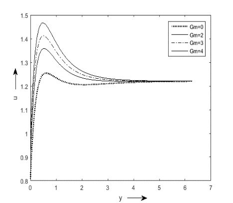
Velocity of fluid flow for distinct values of Gm and Gr are drawn in the Figures (3) and (4). It is noted that the increasing values of Gm and Gr help to improve the velocity. For both thermal and solutal Grasshoff number, buoyancy force dominates the viscous force which gives higher velocity. The results agree well with the study of Prakash et. al. [5].
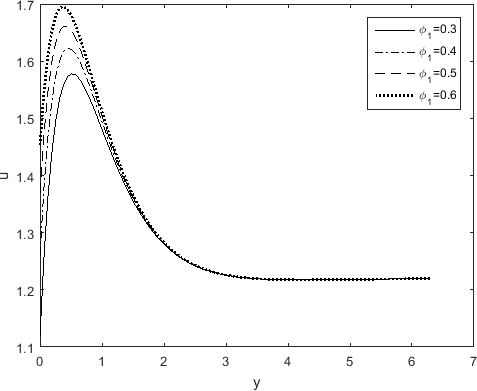
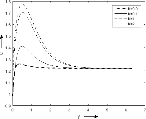
From Figures (5) and (6), the effects of porous permeability parameters K and Ø1 on velocity are observed. Here, Ø1 is directly proportional to the square root of K. In the present study higher permeability K allows the fluids to flow rapidly. As a result, increasing values of Ø1 also enhance the fluid velocity. At K=0.001, we get approximately linear flow after some elevation.
Figure 2. Velocity profiles for Ec, Sc=0.6, F=2, M=2, Gr=4, Gm=2, t=1, Pr=0.2, A=0.5, n1=0.1, Q1=2, Du=0.5,K=0.1
Figure 3. Velocity profiles for Gm, Sc=0.6, F=2, M=2, Gr=4, A=0.5, n1=0.1, t=1, Pr=0.2,K=0.1, Q1=2, Du=0.5
Figure 4. Velocity profiles for Gr, Sc=0.6, F=2, M=2, Gm=2, n1=0.1, t=1, Pr=0.2, K=0.1, A=0.5, Q1=2, Du=0.5
Figure 5. Velocity profiles for Ø1, Sc=0.6, F=2, M=2, Gr=4, Gm=2, n1=0.1, t=1, Pr=0.2,K=0.1, A=0.5, Q1=2, Du=0.5
Figure 6. Velocity profiles for K, Sc=0.6, F=2, M=2, Gm=2, n1=0.1, t=1, Pr=0.2, Gr=4, A=0.5, Q1=2, Du=0.5
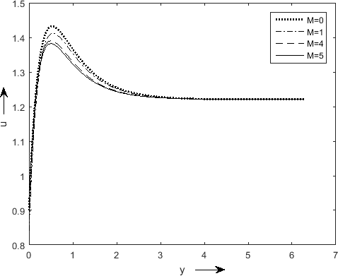
Figure 7. Velocity profiles for M, Sc=0.6, F=2, K=0.1, Gm=2, n1=0.1, t=1, Pr=0.2, Gr=4, A=0.5, Q1=2, Du=0.5, F=2
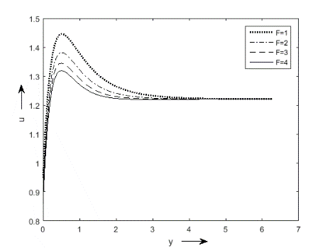
Figure 8. Velocity profiles for F, Sc=0.6, M=2, Gr=4, Gm=2, n1=0.1, t=1, Pr=0.2, K=0.1, Q1=2, Du=0.5, A=0.5
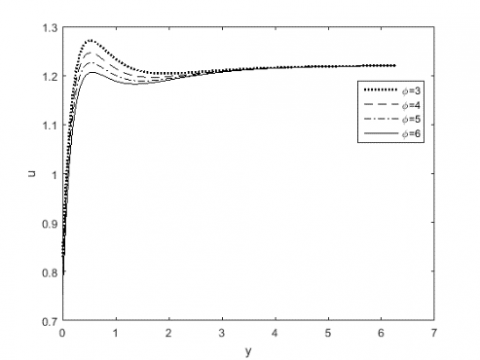
Figure 9. Velocity profiles for Ø, Sc=0.6, M=2, Gr=4, Gm=2, n1=0.1, t=1, Pr=0.2, K=0.1, Q1=2, Du=0.5, A=0.5, F=2
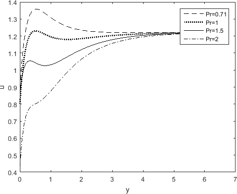
Figure 10. Velocity profiles for Pr, Sc=0.6, M=2, Gr=4, Gm=2, n1=0.1, t=1, K=0.1, Gr=4, Q1=2, Du=0.5, A=0.5, F=2
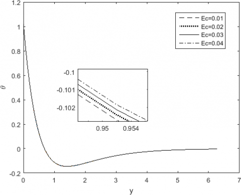
Figure 11. Temperature profiles for Ec, Sc=0.6, M= 2, Gr=4, Gm=2, n1=0.1, t=1, K=0.1, Pr=0.2, Q1=2, Du=0.5, A=0.5, F=2
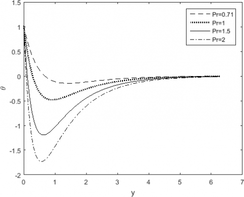
Figure 12. Temperature profiles for Pr, Sc=0.6, M=2, Gr=4, Gm=2, n1=0.1, t=1, K=0.1, F=2, Q1=2, Du=0.5, A=0.5
Table 1. Comparison between present results with previous results
|
γ |
Result of Kim [18] |
Result of Prakash et al. [6] |
Present results |
|||
|
|
Nu |
Sh |
Nu |
Sh |
Nu |
Sh |
|
0.00 |
-1.3400 |
-0.8098 |
-1.3400 |
-0.8098 |
-1.3400 |
-0.8097 |
|
0.50 |
-1.4825 |
-1.1864 |
-1.4825 |
-1.1864 |
-1.4827 |
-1.1859 |
|
0.75 |
-1.5227 |
-1.3178 |
-1.5227 |
-1.3178 |
-1.5227 |
-1.3177 |
|
1.00 |
-1.5546 |
-1.4325 |
-1.5546 |
-1.4325 |
-1.5543 |
-1.4326 |
Figure 7 shows that magnetic parameter acts as a resistive force to the fluid flow. This results also agree well with previous study of Prakash et al. [5].
Figure 8 and 9, that velocity decreases when radiation parameter F and heat absorption parameter Ø increase. So, we can control the flow of fluid by rising both the parameters.
In the Figure 10, effects of Prandtl number (Pr) on velocity is shown. Velocity is reduced with increasing values of Prandtl number. Here the momentum diffusivity influences behaviour of the fluid flow resulting lower velocity.
The increasing values of Eckert number (Ec) lead higher temperature which is shown in Figure 11. But in Figure 12, the Prandtl number (Pr) adversely affects the temperature. Here we can measure the relative importance of viscous dissipation to the thermal dissipation.
Table 2. Values of Nu and $\tau$ w.r.t. Ec
|
Ec |
Nu |
$\tau$ |
|
0.00 |
-0.8243 |
2.3054 |
|
0.01 |
-0.8301 |
2.2896 |
|
0.02 |
-0.8359 |
2.2580 |
|
0.03 |
-0.8416 |
-1.4325 |
|
0.04 |
-0.8474 |
2.2422 |
In Table 1, our results with Ec=0, Sc=0.6, F=2, M=2, Gr=4, Gm=2, Q1=2, Pr=0.2, A=0.5, Du=0.5, n1=0.1, t=1, K=0.1 is compared with the previous results of Prakash et.al. [6], and Kim [18] and it agrees well. This supports our method and accuracy of calculation. From Table 2, the Nusselt number and Skin friction both diminish with higher Eckert number.
The study of viscous dissipation effect on the unsteady MHD flow of an incompressible viscous fluid over a vertical permeable surface fixed in a porous medium is executed in the proximity of thermal radiation and chemical reaction. After applying the perturbation technique, the governing partial differential equations lead some non-linear ordinary differential equations. To handle these non-linearities, Eckert number (Ec) is taken as a small parameter to perturb the equations again. This assumption gives us better result. Some results are given below.
We are thankful to the editors and reviewers for their kind suggestion to improve the manuscript.
|
A |
Suction velocity parameter |
|
B0 |
Magnetic field of uniform strength |
|
C* |
Species concentration, kgm-3 |
|
Cw Cp CS Cf C∞ D Du Dm Ec F Gr Gm g K KT Kλw K* M Nu Pr P* Q Q0 Q* Q1 Q1* qr R Sh Sc T T* |
Species concentration at the plate Specific heat at constant pressure, Jkg-1K Concentration susceptibility the plate Skin friction coefficient Species concentration far away from the plate Chemical molecular diffusivity, m2s-1 Dufour number The coefficient of mass diffusivity Eckert number Thermal radiation parameter Thermal Grashof number Solutal Grashof number Acceleration due to gravity, ms-2 Permeability parameter Thermal diffusion ratio Absorption coefficient at the wall The permeability of the porous medium Hartmann number Nusselt number Prandtl number Pressure Heat source parameter Dimensional heat absorption coefficient Sink strength Radiation absorption parameter The coefficient of proportionality for the absorption Radiative heat flux Chemical reaction parameter Sherwood number Schmidt number Fluid temperature Temperature of fluid near the plate, K
|
|
Tw* T∞* Tw T∞
u, v |
Fluid temperature at the surface, K Fluid temperature in the free stream, K Temperature at the wall The free stream dimensional temperature Radiative heat flux Dimensionless velocity component, ms-1 |
|
Greek symbols |
|
|
a |
Fluid thermal diffusivity, m2s-1 |
|
βT βC |
Thermal expansion coefficient, K-1 Concentration expansion coefficient, K-1 |
|
f f1 |
Heat source parameter Porous permeability parameter |
|
Ɵ |
Dimensionless fluid temperature, K |
|
µ |
Dynamic viscosity, kgm-1s-1 |
|
ν σ f1 η τ ρ |
The kinematic viscosity, m2s-1 The fluid-electrical conductivity Permeability parameter Dimensionless normal distance Skin friction coefficient Density of the fluid, kgm-3 |
|
Subscripts |
|
|
w |
Conditions on the wall |
|
∞ |
Free stream condition |
[1] Devi S.P.A., Ganga B. (2009). Effects of viscous and joules dissipation on MHD flow, heat and mass transfer past a stretching porous surface embedded in a porous medium. Nonlinear Analysis: Modelling and Control, 14(3): 303-314. https://doi.org/10.15388/NA.2009.14.3.14497
[2] Murugesan, T., Kumar M.D. (2019). Viscous dissipation and Joule heating effects on MHD flow of a thermo-solutal stratified nanofluid over an exponentially stretching sheet with radiation and heat generation/absorption. WSN, 129: 193-210.
[3] Kumari, K., Goyal, M. (2017). Viscous dissipation and mass transfer effects on MHD oscillatory flow in a vertical channel with porous medium. Advances in Dynamical Systems and Applications, 12(2): 205-216.
[4] Kumar, D.R., Reddy, K.J. (2018). Viscous dissipation and radiation effects on MHD convective flow past A vertical porous plate with injection. International Journal of Engineering Science Invention, 2319-6726.
[5] Rani, T.R., Radhika, T.S.L., Blackledge, J.M. (2017). The effects of viscous dissipation on convection in a porous medium. Mathematica Aeterna, 7(2): 131-145.
[6] Prakash, J., Prasad, P.D., Kumar, R.V.M.S.S.K., Varma, S.V.K. (2016). Diffusion-thermo effects on MHD free convective radiative and chemically reactive boundary layer flow through a porous medium over a vertical plate. Journal of Computational & Applied Research in Mechanical Engineering, 5(2): 111-126. https://doi.org/10.22061/JCARME.2016.429
[7] Jakati, S.V., Raju, B.T., Nargund, A.L., Sathyanarayana, S.B. (2018). The effect of Thermal radiation, viscous dissipation and chemical reaction on MHD boundary-layer flow of nanofluids over a moving surface. IJMET, 9(13): 1140-1154.
[8] Rao, M.E. (2018). The effects of thermal radiation and chemical reaction on MHD flow of a casson fluid over and exponentially inclined stretching surface. IOP Conf. Series: Journal of Physics, 012158. https://doi.org/10.1088/1742-6596/1000/1/012158
[9] Balamurugan, K.S., Ramaprasad, J.L., Kumar Varma, S.V. (2015). Unsteady MHD free convective flow past a moving vertical plate with time dependent suction and chemical reaction in a slip flow regime. Int. Conf. Comp. Heat Mass Transfer, Proced. Eng., 127: 516-523.
[10] Haile, E., Shankar, B. (2014). Heat and mass transfer through a porous media of MHD flow of nanofluids with thermal radiation, Viscous Dissipation and chemical reaction effects. American Chemical Science Journal, 4(6): 828-846. 10.9734/ACSJ/2014/11082
[11] Reddy, G. (2014). Influence of thermal radiation, viscous dissipation and Hall current on MHD convection flow over a stretched vertical flat plate. Ain Shams Engineering Journal, 5(1): 169-175. https://doi.org/10.1016/j.asej.2013.08.003
[12] Jonnadula, M., Reddy, G.M., Venkateswarlu, M. (2015). Influence of thermal radiation and chemical reaction on MHD flow, heat and mass transfer over a stretching surface. Procedia Engineering, 127: 1315-1322.
[13] Makinde O.D., Khan Z.H., Ahmad R., Khan W.A. (2018). Numerical study of unsteady hydromagnetic radiating fluid flow past a slippery stretching sheet embedded in a porous medium, Physics of Fluids, 30: 083601-083607. https://doi.org/10.1063/1.5046331
[14] Makinde, O.D., Khan, W.A., Khan, Z.H. (2016). Analysis of MHD nanofluid flow over a convectively heated permeable vertical plate embedded in a porous medium. Journal of Nanofluids, 5(4): 574-580. https://doi.org/10.1166/jon.2016.1236
[15] Mutuku-Njane, W.N., Makinde, O.D. (2013). Combined effect of buoyancy force and Navier Slip on MHD flow of a nanofluid over a convectively heated vertical porous plate. The Scientific World Journal, 2013: 735643. https://doi.org/10.1155/2013/725643
[16] Swain, B.K., Senapati, N. (2015). The effect of mass transfer on MHD free convective radiating flow over an impulsively started vertical plate embedded in a porous medium. Journal of Applied Analysis and Computation, 5: 18-27. https://doi.org/10.11948/2015002
[17] Uddin, M.S. (2015). Viscous and joules dissipation on mhd flow past a stretching porous surface embedded in a porous medium. Journal of Applied Mathematics and Physics, 3(12): 1710-1725. https://doi.org/10.4236/jamp.2015.312196
[18] Kim, Y.J. (2000). Unsteady MHD convective heat transfer past a semi-infinite vertical moving plate with variable suction. International Journal of Engineering Sciences, 38(8): 833-845. https://doi.org/10.1016/S0020-7225(99)00063-4
[19] Pal, D., Talukdar, B. (2010). Perturbation Analysis of unsteady magneto hydro - dynamic convective heat and mass transfer in a boundary layer slip flow past a vertical permeable plate with thermal radiation and chemical reaction. Communications in Nonlinear Science and Numerical Simulation, 15(7): 1813-1830. https://doi.org/10.1016/j.cnsns.2009.07.011
[20] Cogley, A.C., Vincent, W.G., Giles, S.E. (1968). Differential approximation to radiative heat transfer in a non-grey gas near equilibrium, American Institute of Aeronautics and Astronautics, 6(3): 551-553. https://doi.org/10.2514/3.4538
[21] Pal, D., Biswas, S. (2016). Perturbation analysis of MHD oscillatory flow on connective radiative heat and mass transfer of micropolar fluid in a porous medium with chemical reaction. Engineering Science and Technology, an International Journal, 19(1): 444-462. https://doi.org/10.1016/j.jestch.2015.09.003