Ramavattula Edukondala Nayak | Munagala Venkata Subba Rao | Kotha Gangadhar*
© 2020 IIETA. This article is published by IIETA and is licensed under the CC BY 4.0 license (http://creativecommons.org/licenses/by/4.0/).
OPEN ACCESS
This investigation is performed for exploring the steady boundary layer flow of mixed convective boundary layer flow of non-Newtonian nanofluid over a stretchable sheet with convection heating. Eyring-Powell fluid is considered as working fluid. The impact of heat absorption/generation, Brownian motion and thermophoresis are taken into consideration. Nonlinear ordinary differential equations are derived from governing equations by utilizing the similarity transformations. To get solution SQL method is used. Accuracy of the proposed technique is checked by comparing with numerical approximations of proposed technique and with results available in literature. The study of parametric approach produces the influence of flow, heat and mass transfer processes. The outcomes of proposed study revealed that parameter of Eyring-Powell fluid ԑ reduces the velocity of the flow and thickness of the momentum buoyancy layer for both assisting and opposing flow conditions while it enhances the temperature and concentration profiles for both flow conditions.
Eyring-Powell fluid, nanofluid, buoyancy effects, heat generation/absorption, convective heating
The study of mixed convection, the arrangement of natural and forced convection stream is one of the best transport phenomenon because of outer constraining mechanism and inward volumetric forces. These stream examples are found at the same time attributable to its significance in numerous down to practical applications; in recent years many researchers are showing their enthusiasm to study the mixed convection with chemical reaction. In this connection, Imtiaz et al. [1] examined about the mixed convection flow of nanofluid by taking into consideration of Newtonian heating. Further, Akram et al. [2] considered study on mixed convective heat and mass transfer of non-Newtonian fluid on peristaltic flow in presence of a vertical axi-symetric channel. Further, Mohammad et al. [3] considered a study in presence of vertical porous media about the effect of viscous heating of nanofluid and regular fluid on mixed convective flow.
In the phrase ‘‘Nanofluids’’ is the best use given by the fluid have adjournment of the nano-sized metallic or the non-metallic particles. It is proposed for utilizing nanoparticles is to get planned about thermal characteristics of the base fluid. The involvement of the nanofluids is upgraded heat different can be notable in specifications in further capable cooling systems, consequentially extreme manufactured, the energy saving. Various eventual petition the nanofluids are the pure heat traders, the radiators are in engines, processes the refrigerate systems, and microelectronics and so on. Choi [4] is initiator he had wrapped up on the investigation on nanoparticles in 1995. Further, Xuan and Roetzel [5] had given caution that the flow of the nanofluid tube using dispersal model. Later, Khanafer et al. [6] examined nanofluid study in 2D flow to enhance heat transfer. Further, Nadeem et al. [7] assumed and conformed that in the study of nanofluid Brownian motion and thermophoresis parameters play a greater role in enhancement of temperature. In another issue, Nadeem and Lee [8] studied nanofluid flow of boundary layer in the direction of stretching surface exponentially.
Analysis of boundary layer flow of non-Newtonian fluids over a stretchable surface has a great importance in various fields for example, coal-oil slurries, metal augmentation, metal turning and so on, the liquids of this sort have a one of a kind significance. There are many researchers like Tan and Masuokat [9], Fetecau et al. [10], Hayat et al. [11], Ishaketal [12] are showing their interest to analyze the studies of various types of non-Newtonian fluids from the untold number of decades or even more. The connection between the shear stress and strain rate in such non-Newtonian liquids will in general be complex. To avoid such type of complexity Eyring-Powell fluid are very useful because Eyring-Powell liquid model has an unequivocal favourable position over the other Newtonian liquids its conduct in higher shear stress in like viscous liquid. Aim is tried to this field of research the re-presents earlier regarding Erying-Powell fluid (Powell and Eyring [13]). Satyaban et al. [14] examined about two effects those are Soret and Dufour to characterise heat and mass transfer in the mixed convective flow of boundary layer of Powell-Erying fluid. Further, Malik et al. [15] studied about mixed convection flow of MHD Eyring-Powell nanofluid over a stretchable sheet.
Later on, Javed et al. [16] is investigated about the non-Newtonian fluid flow of Eyring-Powell over a stretchable sheet. Further, Nadeem et al. [17] is investigated about the partial slip impacts on a fourth-grade fluid by means of variable viscosity. Ishak et al. [18] is investigated about the mixed convection flow of micropolar stagnation point fluid flow in the direction of a stretching sheet. Recently, Gangadhar et al. [19] considered convective heating in his study to present the impact of thermal radiation on engine oil nanofluid flow. Futher, Gangadhar et al. [20] used numerical technique that is spectral quasi-linearisation method to present the features of microstructure and inertial characteristic of a magnetite Ferro fluid. Gangadhar et al. [21] studied boundary layer flow of viscous dissipation and variable suction/injection numerically. Further, Gangadhar et al. [22] conducted a numerical study to produce some features about unsteady boundary layer flow of nanofluid. Later on, Gangadhar et al. [23] explored some of the impacts by studying the MHD micropolar nanofluid in presence of Newtonian heating. Venkata Subba Rao et al. [24] conducted numerical study on MHD boundary layer flow of nanofluid.
The particular goal of the present work is to investigate the effect of heat absorption/generation, Brownian motion and thermophoresis in the nanofluid flow of Eyring-Powell liquid by considering mixed convection. Different physical parameters each one of those is associated with the problem are impact the fluid flow and those impacts are inspected by means of the proposed convergent numerical strategy. All those numerical outcomes are shown in graphs and table.
In this study flow is assumed to be two-dimensional, viscous, incompressible electrically conducting, non-Newtonian nanofluid of Eyring-Powell, present study is conducted on stretching sheet. Here, $u_{w}=a x$ is the stretching velocity (Figure 1).
From the above mentioned suppositions governing equations of continuity, momentum, energy and species of the present study is given by
$\frac{\partial u}{\partial x}+\frac{\partial v}{\partial y}=0$ (1)
$\begin{align} & v\frac{\partial u}{\partial y}+u\frac{\partial u}{\partial x}=\left( \upsilon +\frac{1}{\rho \beta c} \right)\left( \frac{{{\partial }^{2}}u}{\partial {{y}^{2}}}+\frac{{{\partial }^{2}}u}{\partial {{x}^{2}}} \right)-\frac{1}{3\rho {{\delta }^{*}}{{c}^{3}}}\frac{\partial }{\partial x}{{\left\{ 2\left( \frac{\partial u}{\partial x} \right) \right.}^{2}}+ \\ & \left. 2{{\left( \frac{\partial v}{\partial y} \right)}^{2}}+{{\left( \frac{\partial u}{\partial y}+\frac{\partial v}{\partial x} \right)}^{2}} \right\}\frac{\partial u}{\partial x}-\frac{1}{6\rho {{\delta }^{*}}{{c}^{3}}}\frac{\partial }{\partial y}{{\left\{ 2\left( \frac{\partial u}{\partial x} \right) \right.}^{2}}+2{{\left( \frac{\partial v}{\partial y} \right)}^{2}}+ \\ & \left. \,\,\,\,\,\,\,\,\,\,\,\,\,{{\left( \frac{\partial u}{\partial y}+\frac{\partial v}{\partial x} \right)}^{2}} \right\}\left( \frac{\partial u}{\partial y}+\frac{\partial v}{\partial x} \right)\pm \frac{g{{\beta }_{0}}(T-{{T}_{\infty }})}{\rho }\pm \frac{g{{\beta }_{1}}(C-{{C}_{\infty }})}{\rho }, \\\end{align}$ (2)
$\begin{align} & v\frac{\partial v}{\partial y}+u\frac{\partial v}{\partial x}=\left( \upsilon +\frac{1}{\rho \beta c} \right)\left( \frac{{{\partial }^{2}}v}{\partial {{y}^{2}}}+\frac{{{\partial }^{2}}v}{\partial {{x}^{2}}} \right)-\frac{1}{6\rho {{\delta }^{*}}{{c}^{3}}}\frac{\partial }{\partial x}{{\left\{ 2\left( \frac{\partial u}{\partial x} \right) \right.}^{2}}+ \\ & \left. 2{{\left( \frac{\partial v}{\partial y} \right)}^{2}}+{{\left( \frac{\partial u}{\partial y}+\frac{\partial v}{\partial x} \right)}^{2}} \right\}\left( \frac{\partial u}{\partial y}+\frac{\partial v}{\partial x} \right)-\frac{1}{3\rho {{\delta }^{*}}{{c}^{3}}}\frac{\partial }{\partial y}{{\left\{ 2\left( \frac{\partial u}{\partial x} \right) \right.}^{2}}+2{{\left( \frac{\partial v}{\partial y} \right)}^{2}} \\ & \left. \,\,\,\,\,\,\,\,\,\,\,\,\,\,\,\,\,\,\,\,\,\,\,\,\,\,\,\,\,\,\,\,\,\,\,\,+{{\left( \frac{\partial u}{\partial y}+\frac{\partial v}{\partial x} \right)}^{2}} \right\}\frac{\partial v}{\partial y}\pm \frac{g{{\beta }_{0}}(T-{{T}_{\infty }})}{\rho }\pm \frac{g{{\beta }_{1}}(C-{{C}_{\infty }})}{\rho }, \\\end{align}$ (3)
$\begin{align} & \left. \left. \,\,\,\,\,\,\,\,\,\,\,\,\,\,\,\,\,\,\frac{\partial C}{\partial y}\frac{\partial T}{\partial y} \right)+\left( \frac{{{D}_{T}}}{{{T}_{\infty }}} \right)\left[ {{\left( \frac{\partial T}{\partial x} \right)}^{2}}+{{\left( \frac{\partial T}{\partial y} \right)}^{2}} \right] \right\}+\frac{{{q}_{0}}}{\rho {{c}_{p}}}(T-{{T}_{\infty }}), \\\end{align}$ (4)
$v\frac{\partial C}{\partial y}+u\frac{\partial C}{\partial x}=\alpha \left( \frac{{{\partial }^{2}}C}{\partial {{y}^{2}}}+\frac{{{\partial }^{2}}C}{\partial {{x}^{2}}} \right)+\left( \frac{{{D}_{T}}}{{{T}_{\infty }}} \right)\left[ \frac{{{\partial }^{2}}T}{\partial {{x}^{2}}}+\frac{{{\partial }^{2}}T}{\partial {{y}^{2}}} \right]$ (5)
Figure 1. Physical sketch of the problem
The following are the boundary conditions for the concentration, velocity and temperatures of the study
$\begin{align} & u={{u}_{w}}(x)=ax,\,\,v=0,\,\, \\ & \,\,\,\,\,\,\,\,\,\,\,\,-k\left( \frac{\partial T}{\partial x}+\frac{\partial T}{\partial y} \right)={{h}_{f}}\left( {{T}_{f}}-T \right),\,\,C={{C}_{w}}, \\\end{align}$at$y=0,$ (6)
$u\to 0,\,\,T\to {{T}_{\infty }},C\to {{C}_{\infty }},$as $y\to \infty ,$ (7)
where, $u$ and $v$ refer to velocity segments in the direction of $x$ and $y$ axes in order, $T_{\infty}$ refer to free stream temperature, $\alpha$ refer to thermal diffusivity, $T$ refer to fluid temperature, $T_{f}$ refer to temperature of the hot fluid, $\mu$ refer to dynamic viscosity fluid, $D_{B}$ refer to Brownian diffusion coefficient, $D_{T}$ refer to thermophoresis diffusion coefficient, $v=\frac{\mu}{\rho}$ refer to kinematic viscosity, $\tau$ refer to ratio of effectual heat capacity of the fluid, $\rho$ refer to density, $\delta$ refer to fluid parameter, $\sigma$ refer to electrically conductivity of the fluid, $B_{0}$ refer to thermal buoyancy coefficient and $\beta_{1}$ refer to mass buoyancy coefficient, $h_{f}$ refer to coefficient of heat transfer and $C$ refer to coefficient of volumetric volume expansion. By applying the boundary layer estimations, Eqns. (2)-(6) can be expressed as follow:
$\begin{align} & v\frac{\partial u}{\partial y}+u\frac{\partial u}{\partial x}=\left( \upsilon +\frac{1}{\rho \beta c} \right)\frac{{{\partial }^{2}}u}{\partial {{y}^{2}}}-\frac{1}{2\rho {{\delta }^{*}}{{c}^{3}}}{{\left( \frac{\partial u}{\partial y} \right)}^{2}}\frac{{{\partial }^{2}}u}{\partial {{y}^{2}}} \\ & \,\,\,\,\,\,\,\,\,\,\,\,\,\,\,\,\,\,\,\,\,\,\,\,\,\,\,\,\,\,\,\,\,\,\,\,\,\,\,\,\,\,\,\,\,\,\,\,\,\,\,\,\,\,\,\,\,\,\,\,\,\pm \frac{g{{\beta }_{0}}(T-{{T}_{\infty }})}{\rho }\pm \frac{g{{\beta }_{1}}(C-{{C}_{\infty }})}{\rho }, \\\end{align}$ (8)
$\begin{align} & v\frac{\partial T}{\partial y}+u\frac{\partial T}{\partial x}=\alpha \left( \frac{{{\partial }^{2}}T}{\partial {{y}^{2}}} \right)+\tau \left\{ {{D}_{B}}\left( \frac{\partial C}{\partial y}\frac{\partial T}{\partial y} \right. \right.+\left. \left( \frac{{{D}_{T}}}{{{T}_{\infty }}} \right){{\left( \frac{\partial T}{\partial y} \right)}^{2}} \right\} \\ & \,\,\,\,\,\,\,\,\,\,\,\,\,\,\,\,\,\,\,\,\,\,\,\,\,\,\,\,\,\,\,\,\,\,\,\,\,\,\,\,\,\,\,\,\,\,\,\,\,\,\,\,\,\,\,\,\,\,\,\,\,\,\,\,\,\,\,\,\,\,\,\,\,\,\,\,\,\,\,\,\,\,\,\,\,\,\,\,+\frac{{{q}_{0}}}{\rho {{c}_{p}}}(T-{{T}_{\infty }}), \\\end{align}$ (9)
$v\frac{\partial C}{\partial y}+u\frac{\partial C}{\partial x}=\alpha \left( \frac{{{\partial }^{2}}C}{\partial {{y}^{2}}} \right)+\left( \frac{{{D}_{T}}}{{{T}_{\infty }}} \right)\left[ \frac{{{\partial }^{2}}T}{\partial {{y}^{2}}} \right]$ (10)
Boundary conditions are as follow:
$\begin{align} & u={{u}_{w}}(x)=ax,\,\,v=0,\,\, \\ & -k\frac{\partial T}{\partial y}={{h}_{f}}\left( {{T}_{f}}-T \right),\,\,C={{C}_{w}}, \\\end{align}$at$y=0,$ (11)
$u\to 0,\,\,T\to {{T}_{\infty }},C\to {{C}_{\infty }},$as $y\to \infty ,$ (12)
The following are the similarity transformations
$\begin{align} & \psi ={{\left( a\upsilon \right)}^{1/2}}x\,f\left( \xi \right),\,\,\theta \left( \xi \right)=\frac{T-{{T}_{\infty }}}{{{T}_{f}}-{{T}_{\infty }}},\,\phi \left( \xi \right)=\frac{C-{{C}_{\infty }}}{{{C}_{w}}-{{C}_{\infty }}},\, \\ & \xi ={{\left( \frac{a}{\upsilon } \right)}^{1/2}}y,\,\,u=ax\,{f}'\left( \xi \right),\,\,v=-\sqrt{a\upsilon }\,f\left( \xi \right), \\\end{align}$ (13)
here, $\psi $ be the stream function, $u=\frac{\partial \psi }{\partial y},\,v=-\frac{\partial \psi }{\partial x}$.
With the help of above mentioned assumptions Eqns. (8)-(12) can be written as
$\left( 1+\omega \right){{{f}'}'}'-{{{f}'}^{2}}+f\,{{f}'}'-\omega \,\lambda \,{{{{f}'}'}^{2}}{{{f}'}'}'\pm \beta \,\theta \pm \delta \,\phi ,$ (14)
$\frac{1}{\Pr }{{\theta }'}'+f\,{\theta }'+Nb\,{\phi }'\,{\theta }'+Nt\,{{{\theta }'}^{2}}+Q\,\theta =0,$ (15)
${{\phi }'}'+\Pr \,Le\,f\,{\phi }'+\frac{Nt}{Nb}{{\theta }'}'=0,$ (16)
Similarly transformed boundary conditions can be expressed
$\begin{align} & f(0)=0,\,{f}'(0)=1,\, \\ & {\theta }'(0)=-Bi\,(1-\theta (0)),\,\phi (0)=1, \\\end{align}$ (17)
${f}'(\infty )\to 0,\,\theta (\infty )\to 0,\,\,\phi (\infty )\to 0,$ (18)
where, prime symbolize diff. w. r. to $\xi $.
$\omega =\frac{1}{\mu {{\delta }^{*}}c}$ and $\lambda =\frac{{{a}^{3}}{{x}^{2}}}{2{{c}^{2}}\upsilon }$ are fluid parameters,$\beta =\frac{g{{\beta }_{0}}({{T}_{w}}-{{T}_{\infty }})}{\rho a}$ the thermal buoyancy parameter,$\delta =\frac{g{{\beta }_{1}}({{C}_{w}}-{{C}_{\infty }})}{\rho a}$ is the mass buoyancy parameter and $\Pr =\frac{\upsilon }{\alpha }$be the Prandtl number, $Le=\frac{\alpha }{{{D}_{B}}}$is Lewis number, $Nt=\frac{\tau {{D}_{T}}({{T}_{f}}-{{T}_{\infty }})}{\upsilon {{T}_{\infty }}}$ is thermophoresis parameter,$Nb=\frac{\tau {{D}_{B}}({{C}_{w}}-{{C}_{\infty }})}{\upsilon }$refer to parameter of Brownian movement, $Bi=\frac{{{h}_{f}}}{k}{{\left( \frac{\upsilon }{a} \right)}^{1/2}}$refer to local Biot number, $\psi $refer to temperature generation ($Q>0$) and temperature absorption ($Q<0$) parameter.
Parameters of noteworthy attentiveness are available problem the local Nusselt number $N{{u}_{x}}$ local Sherwood number $S{{h}_{x}}$ and skin-friction coefficient ${{C}_{fx}}$,
${{C}_{fx}}=\frac{{{\tau }_{w}}}{\rho u_{w}^{2}},\,N{{u}_{x}}=\frac{x{{q}_{w}}}{k({{T}_{f}}-{{T}_{\infty }})},S{{h}_{x}}=\frac{x{{q}_{m}}}{{{D}_{B}}({{C}_{w}}-{{C}_{\infty }})},$ (19)
Here heat and mass transfer from the surface are denoted with ${{q}_{w}}$ and $q_{m}$ respectively, local shear stress at wall denoted with $τ_w$ and all these are follows as below:
$\begin{align} & {{\tau }_{w}}={{\left[ \left( 1+\frac{1}{{{\delta }^{*}}c} \right)\frac{\partial u}{\partial y}-\frac{1}{6{{\delta }^{*}}{{c}^{3}}}{{\left( \frac{\partial u}{\partial y} \right)}^{3}} \right]}_{y=0}}, \\ & {{q}_{w}}=-k{{\left[ \frac{\partial T}{\partial y} \right]}_{y=0}}, \\ & {{q}_{m}}=-{{D}_{B}}{{\left[ \frac{\partial C}{\partial y} \right]}_{y=0}}, \\\end{align}$ (20)
By means of above defined similarity transformations the skin friction coefficient, the local Sherwood number and Nusselt number can be expressed as follows:
$\begin{align} & Re_{x}^{1/2}{{C}_{fx}}=\left[ \left( 1+\omega \right){{f}'}'(0)-\frac{\lambda }{3}{{{{{f}'}'}}^{3}}(0) \right], \\& Re_{x}^{-1/2}N{{u}_{x}}=-{\theta }'(0), \\& Re_{x}^{-1/2}S{{h}_{x}}=-{\phi }'(0), \\\end{align}$ (21)
where, $R{{e}_{x}}=\frac{x{{u}_{w}}}{\upsilon }$ is the Reynolds number.
Spectral quasi linearization method is used to solve the transformed differential Eqns. (14)-(16) subjected to the suitable boundary conditions (17)-(18). Actually, this method is proposed by Bellman and Kalaba [25]. Thereafter, it follows generalization method of Newton Raphson. So that Eqns. (14)-(16) are followed as:
$\,{{a}_{1r}}\,\,{{{f}'''}_{r+1}}\,\,+\,\,{{a}_{2r}}\,{{{f}''}_{r+1}}\,\,\pm \,\,\beta \,\,{{\theta }_{r+1}}\,\,\pm \,\,\delta \,{{\varphi }_{r+1}}\,=\,\,\,{{R}_{1,r}},$
$\frac{1}{\Pr }\,\,{{{{\theta }'}'}_{r+1}}\,\,+\,\,{{b}_{1r}}\,\,{{{\theta }'}_{r+1}}\,\,+\,\,\varphi \,{{\theta }_{r+1}}\,\,=\,\,{{R}_{2,r\,}},$ (22)
${{{{\varphi }'}'}_{r+1}}\,\,+\,\,{{c}_{1r}}\,\,{{{\varphi }'}_{r+1}}\,\,\,=\,\,\,{{R}_{3,r\,}},$
here,$\,{{a}_{s1}},\,\,r\,(\,{{s}_{1}}\,\,=\,\,1,\,\,2\,),\,\,{{b}_{1r}},\,\,{{c}_{1r}}$are known functions, moreover all these are defined as
${{a}_{1r}}\,\,=\,\,1\,\,+\,\,\varepsilon \,\,-\,\,\varepsilon \,\lambda \,{{f}_{r}}{{^{\prime }}^{\prime }}^{2},$
${{a}_{2r}}\,=\,\,{{f}_{r}},$
${{R}_{1r}}\,\,=\,\,{{f}_{r}}{{^{\prime }}^{2}}\,,$
${{b}_{1r}}\,\,=\,\,{{f}_{r}}\,\,+\,\,Nb\,\,{{{\varphi }'}_{r}},$
${{R}_{2r}}\,\,=\,\,-\,\,Nt\,\,{{{\theta }'}_{r}}^{2}\,\,,$
${{C}_{1r}}\,\,=\,\,{{P}_{r}}\,\,Le\,{{f}_{r}}\,,$
${{R}_{3r}}\,\,=\,\,-\,\,\frac{Nt}{Nb}\,\,{{\varphi }_{r}}^{\prime\prime }\,\,,$ (23)
${{f}_{r+1}}\,\,(0)\,\,=\,\,0,$
${{{f}'}_{r+1}}\,\,(0)\,\,=\,\,\,1,$
${{{f}'}_{r+1}}\,\,(\infty )\,\,=\,\,0,$
${{{\theta }'}_{r+1}}\,\,\,(0\,)\,\,=\,\,-\,\,Bi\,\,(\,1-{{\theta }_{r+1}}\,(\,0\,)\,)\,,$
${{\theta }_{r+1}}\,\,(\infty )\,\,=\,\,0\,,$
$\begin{align} & {{\varphi }_{r+1}}\,\,(\,0\,)\,\,=\,\,1\,, \\ & {{\varphi }_{r+1}}\,\,(\,\infty \,)\,\,\,=\,\,0\,. \\\end{align}$ (24)
The bunch of equations in (22) is known as coupled linear differential equations with variable coefficients. From that point one of the realized numerical techniques is utilized to illuminate set of equations with the approximation method by taking r=1, 2, 3, 4…....
Thereafter Chebyshev pseudo spectral method is utilized to apply the QLM scheme (22)
${{f}_{0}}\left( \xi \right)=1-{{e}^{-\xi }},\,\,\,{{\theta }_{0}}\left( \xi \right)=\frac{{{B}_{i}}}{1+{{B}_{i}}}{{e}^{-\xi }},\,\,\,{{\varphi }_{0}}\left( \xi \right)={{e}^{-\xi }}\,.$ (25)
If initial approximations ${{f}_{0}}$, ${{\theta }_{0}}$ and ${{\varphi }_{0}}$ the iteration schemes (31) is iteratively for${{f}_{r+1}}\,(\xi )$,${{\theta }_{r+1}}\,(\xi )$ and${{\varphi }_{r+1}}\,(\xi $), here r=1,2,3,4…, we discretize the equation to use chebyshev spectral collocation method. The evaluate unrevealed amount engage the Chebyshev interpolating polynomials and collocated at the Gauss-Lobatto collocation points is
${{t}_{j}}\,=\,\,\cos \,\,\frac{\pi j}{N},\,$ j = 0, 1, 2, 3, ….., $\bar{N}$. (26)
where, $\bar{N}$ refer to number of collocation points. And the real domain [0,$\infty $) is convert in to [-1, 1] on applying the domain truncation capability. The problem is resolved interregnum [0,${{\xi }_{\infty }}$] rather of [0,$\infty \,]$. This conduct to mapping
$\frac{\xi }{{{\xi }_{\infty 2}}}\,\,=\,\,\frac{\tau +1}{2},\,\,$ -1$\,\,\le \,\,\tau \,\,\le \,\,1$, (27)
where, ${{\xi }_{\infty }}$ is the escalating parameter is applying to entreat the boundary conditions at $\infty $. The $f$, θ, and δ of approximate values and the collocation points are written by
$f\,\,(\tau )\,\,=\,\,\sum\limits_{k=0}^{{\bar{N}}}{\,f\,\,(\,{{\tau }_{k}})\,\,{{T}_{k}}\,({{\tau }_{j}})},$
$\theta \,\,(\tau )\,\,=\,\,\sum\limits_{k=0}^{{\bar{N}}}{\,\theta \,\,(\,{{\tau }_{k}})\,\,{{T}_{k}}\,(\,{{\tau }_{j}})},$
$\varphi \,\,(\,\tau )\,\,=\,\,\sum\limits_{k=0}^{{\bar{N}}}{\,\,\varphi \,\,(\,{{\tau }_{k}})\,\,{{T}_{k}}\,({{\tau }_{j}})},$ (28)
here, ${{T}_{K}}$is the k$^{th}$Chebyshev polynomial state
${{T}_{k}}(\tau )\,\,\,=\,\cos \,\,\left[ k\,{{\cos }^{-1}}\,(\tau )\, \right]$. (29)
The derivative of variable is establishing
$\frac{{{d}^{p}}f}{d{{\xi }^{p}}}\,\,\,=\,\,\,\sum\limits_{k=0}^{{\bar{N}}}{\,\,D\,_{lk}^{p}\,f\,(\,{{\tau }_{k}})}$
$\frac{{{d}^{p}}\theta }{d{{\xi }^{p}}}\,\,\,=\,\,\sum\limits_{k=0}^{{\bar{N}}}{\,\,D\,_{lk}^{p}\,\theta \,\,(\,{{\tau }_{k}})}$
$\frac{{{d}^{p}}\varphi \,\,}{d{{\xi }^{p}}}=\,\,\sum\limits_{k=0}^{{\bar{N}}}{\,D\,_{lk}^{p}\,\varphi \,\,(\,{{\tau }_{k}})}$, where, l=0, 1, 2, 3, 4…$\bar{N}$(30)
In bunch of Eq. (30), p refers to order of derivative. Differentiation matrix of chebyshev spectral method is dented by D and defined as $D\,\,=\,\,\,\frac{2{{D}_{1}}}{{{\xi }_{\infty }}}$ and its related components are clearly finned in Canuto et al. [26]. By substituting the Eqns. (27)-(30) in (22), the following matrix form is obtained
AX = R. (31)
Together with boundary conditions
$\begin{align} & {{f}_{r+1}}\,({{\tau }_{{\bar{N}}}})\,\,=\,\,0, \\ & \sum\limits_{k=0}^{{\bar{N}}}{\,{{D}_{\bar{N}K}}\,f\,({{\tau }_{k}})\,\,=\,\,1,} \\\end{align}$
$\sum\limits_{k=0}^{{\bar{N}}}{\,{{D}_{0k}}\,f\,({{\tau }_{k}})\,\,=\,\,0,}$
$\sum\limits_{k=0}^{{\bar{N}}}{\,{{D}_{\bar{N}k}}\,\theta \,({{\tau }_{k}})\,\,=\,\,-Bi\,(1-{{\theta }_{r+1}}\,({{\tau }_{{\bar{N}}}})\,)},$
$\begin{align} & {{\theta }_{r+1}}\,({{\tau }_{0}})\,\,=\,\,0, \\ & {{\varphi }_{r+1}}\,({{\tau }_{{\bar{N}}}})\,\,=\,\,1, \\ & {{\varphi }_{r+1}}\,\,({{\tau }_{0}})\,\,\,=0. \\\end{align}$ (32)
In the Eq. (31), A refer to square matrix with size $(3\bar{N}+3)\times (3\bar{N}+3)$, X and R refer to column vector with size $\left( 3\bar{N}+3 \right)\times 1$ and these are given as below
$A=\left[ \begin{matrix} {{A}_{11}} & {{A}_{12}} & {{A}_{13}} \\ {{A}_{21}} & {{A}_{22}} & {{A}_{23}} \\ {{A}_{31}} & {{A}_{32}} & {{A}_{33}} \\\end{matrix} \right]$,$X=\left[ \begin{matrix} {{f}_{r+1}} \\ {{\theta }_{r+1}} \\ {{\varphi }_{r+1}} \\\end{matrix} \right]$,$R=\left[ \begin{matrix} {{R}_{1}} \\ {{R}_{2}} \\ {{R}_{3}} \\\end{matrix} \right]$, (33)
where, $f\,\,=\,\,{{\left[ \,{{f}_{r+1}}\,({{\tau }_{0}}),\,\,{{f}_{r+1}}\,({{\tau }_{1}}),\,\,{{f}_{r+1}}\,({{\tau }_{2}})\,,\,.\,.\,.\,.\,.\,...\,.\,,\,{{f}_{r+1}}\,({{\tau }_{{\bar{N}}}})\, \right]}^{T}}$, $\theta \,\,=\,\,{{\left[ \,{{\theta }_{r+1}}\,({{\tau }_{0}}),\,\,{{\theta }_{r+1}}\,({{\tau }_{1}}),\,\,{{\theta }_{r+1}}\,({{\tau }_{2}}),\,.\,.\,.\,.\,.\,.\,.\,.\,.\,,\,{{\theta }_{r+1}}\,({{\tau }_{{\bar{N}}}})\, \right]}^{T}}$, $\varphi \,\,=\,\,{{\left[ \,{{\varphi }_{r+1}}\,({{\tau }_{0}}),\,\,{{\varphi }_{r+1}}\,({{\tau }_{1}}),\,\,{{\varphi }_{r+1}}\,({{\tau }_{2}}),\,.\,.\,.\,..\,.\,..\,,\,\,{{\varphi }_{r+1}}\,({{\tau }_{{\bar{N}}}})\, \right]}^{T}}$, $A_{11}=\operatorname{diag}\left[a_{2 r}\right] D^{3}+\operatorname{diag}\left[a_{2 r}\right] D$, ${{A}_{12}}\,\,\,=\,\,\pm \,\,\beta I\,,$ ${{A}_{13}}\,\,\,=\,\,\pm \,\,\delta I\,,$ ${{A}_{21}}\,\,\,=\,\,0\,,$ ${{A}_{22}}\,\,\,=\,\,\frac{1}{\Pr }\,\,{{D}^{2}}\,\,+\,\,diag\,\left[ {{b}_{1r}} \right]\,D\,\,+\,\,\varphi I\,,$ ${{A}_{23}}\,\,\,=\,\,\,0\,,$ ${{A}_{31}}\,\,\,=\,\,\,0\,,$ ${{A}_{32}}\,\,\,=\,\,\,\,0\,,$ ${{A}_{33}}\,\,\,=\,\,{{D}^{2}}\,+\,diag\,\left[ {{c}_{1r}} \right]\,\,D\,,$ ${{R}_{1}}\,\,\,\,\,=\,\,\,\,{{R}_{1,r}}\,,$ ${{R}_{2}}\,\,\,\,\,=\,\,\,{{R}_{2,r}}\,,$ ${{R}_{3}}\,\,\,\,\,=\,\,\,\,{{R}_{3,r}}\,,$, and here I refer to identity matrix, O refer to column matrix of the order $\left( \,\bar{N}+1\, \right)\,\,\times \,\,1,\,$diag[ ] refer to diagonal matrix with the order $\left( \,\bar{N}+1\, \right)\,\,\times \,\,\left( \,\bar{N}+1\, \right).\,$Subscript r is used to represent the iteration number. After improving the matrix system Eq. (22) together with boundary condition (32), then solution can be obtained in the form of
$X\,\,=\,\,{{A}^{-1}}\,R\,$. (34)
In this section all the numerical outcomes are exposed graphically from Figure 2 to Figure 21 to talk about different resulting parameters encountered in the present study. The results which are acquired from the numerical strategy talked about in the past segment are contrasted and those of Rashidi et al. [27] and wang [28] and showed in Table 1. This correlation demonstrates a good understanding between present examination and past investigations. Moreover, the results show that the Spectral Quasi Linearization Method is productive and sufficiently amazing for utilization of taking care of solving fluid flow problems.
Table 1. Comparison between present study wall heat transfer rate $-\theta^{\prime}(0)$ with the existing outcomes in literature for various values of $P r$ when $\varepsilon=\delta=\beta=Q=N t=N b=0$ and $B i \rightarrow \infty$
|
$-\theta^{\prime}(0)$ |
|
||
|
Pr |
Present study |
Rashidi et al. [27] |
Wang [28] |
|
2.0 7.0 |
0.91135768 1.89540327 |
0.91135769 1.89540340 |
0.91136 1.89540 |
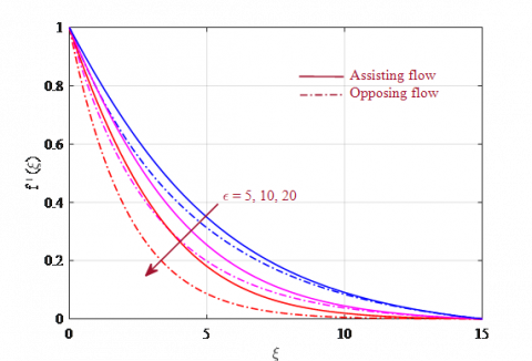
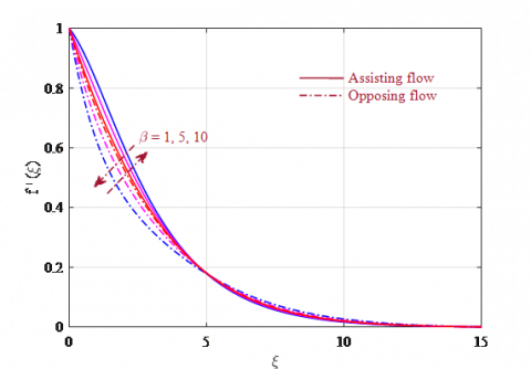
Figure 2,3 and 4 depict velocity distribution $f^{\prime}(\xi)$ with increasing of Eyring-Powell fluid parameter $\varepsilon,$ thermal buoyancy parameter $\beta,$ and mass buoyancy parameter $\delta$ for both assisting and opposing flows. From Figure $2,$ is observed that the velocity profile and momentum buoyancy layer thickness is enhanced as $\varepsilon$ increasing in both flow conditions. This is all only the cause of Powell-Eyring fluids are share thinning fluid the velocity gets low at the share rate increases. Also, it is mentioned that velocity distribution for assisting flow is high compare to opposing flow. Figure 3 present the curves of the velocity profile for various values $\beta$ and at fixed values of other parameters. The gradual is increase in the parameter $\beta$ shows stronger thermal buoyancy force which leads to high velocity. This is because, positive $\beta$ used as flattering pressure gradient for fluid flow near the surface attributable to which $f^{\prime}(\xi)$ is huge. Again, an overshoot in contour is can be seen only for huge values of $\beta .$ The opposite manner is observed for negative $\beta,$ In Figure $4,$ the curves of $f^{\prime}(\xi)$ for difference of mass buoyancy parameter $\delta$ are presented at specific values of other parameters. We had checked that the function $f^{\prime}(\xi)$ increases with the increase in δ in that occurrence the aiding flow and the reversal trend is observed for opposite flow criteria.
Figure 2. Graph for velocity distribution for different values of $\varepsilon$
Figure 3. Graph for velocity distribution for various values of $\beta$
Figure 4. Graph for velocity distribution for various values of $\delta$
Figure 5. Graph for temperature distribution for various values of $\varepsilon$
Figure 6. Graph for temperature distribution for various values of $\beta$
Figure 7. Graph for temperature distribution for various values of $\delta$
Figures 5, 6, 7, 8, 9, 10, 11 and 12 depict temperature distribution $\theta(\xi)$ with increasing of Eyring-Powell fluid parameter $\varepsilon,$ thermal buoyancy $\beta,$ mass buoyancy $\delta$ thermophoresis $N t,$ Brownian motion $N b,$ heat source/sink $Q,$ Biot number $B$ iand Prandtl number $P r .$ The Figure $5,$ shows that the recovered for higher values on Eyring-Powell fluid parameter $\varepsilon,$ and the heat of fluid rises. Then the cause beyond that incremental values of parameter $\varepsilon$ assist at increasing with heat generation which in turn construct heat with in the fluid which in return increases the median kinetic energy of the molecules for one and the other assisting and opposing flow conditions. The Figure 6, was noticed that the thermal buoyancy layer thickness and the temperature transmission percentage is decreases with the rise $P r$ the assisting flow and reveres trend has noticed thatthe opposing flow case.
Figure 8. Graph temperature distribution for various values of Nt
Figure 9. Graph temperature distribution for various values of Nb
Figure 10. Graph for temperature distribution for various values of Q
The behavior of $\delta$ on dimensionless heat is presented in the Figure $7 .$ Is observed that the thickness by thermal buoyancy layer and the heat of the fluid decreases the Figure 8 and opposing for negative $\delta .$ The circumstance of the dispersal of piece, in the presences of heat acclivity, is accepted the thermophoresis. The validation of temperature $\theta(\xi)$ the different rate of $N t$ is present in the Figure $8,$ the augmentation of the value $N t$ causes the temperature gradient of the result in escalating the force (thermophoresis) with nanoparticles. These impacts are superintended by a bit additional fluids existence the heated and upraise at the temperature. The reversible consequence is noticed that occurrence of opposing flow, the Brownian motion is the unsystematic act of the nanoparticles inner side of foundation fluid attributable to the repeated impact of nano particle the particles of paltry fluid. This act of the molecules is defined by the parameter $N b$, is also noted as Brownian motion coefficient.
Figure 11. Graph for temperature distribution for various values of Bi
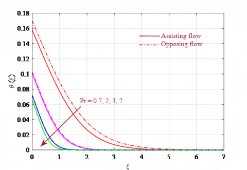
Figure 12. Graph for temperature distribution for various values of Pr
Figure 13. Graph for concentration distribution for various values of $\mathcal{E}$
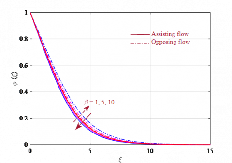
Figure 14. Graph for concentration distribution for various values of $\beta$
Figure 10 shows the enhancement of the temperature generation or absorption parameter $Q$ on the heat distribution. It is apparent that the fluid temperature that goes high with temperature generation $(Q>0) .$ And decreases with the temperature absorption $(Q<0) .$ The physical reason is that the existence of the temperature generation $(Q>0)$ has been effort to increase the thermal state of fluid is the base of its heat and thermal buoyancy layer thickness to increase. The occurrence of the heat absorption $(Q<0)$ both the fluid heat and its thermal buoyancy layer thickness tends to decrease temperature contours, represented by $\theta(\xi),$ are plotted at different rate of Biot number signifies the power of convective heating. Layer Biot number implicit stronger convective heating at the plate attributable to which temperature rises gradually. The occurrence $B i=0$ represents iso-fluxhf wall state while isothermal wall case is jumped as $B i \rightarrow \infty .$ The consequence of Prandtl number is dimensionless temperature the Figure 12 for aiding and opposing flow criteria reciprocally. Then the Prandtl number explain the rate of the momentum diffused to the thermal diffused. HerePr $=1,$ both momentum and thermal diffusivities was equivalent, because the $P r>1$ the momentum diffusivity is considerable than the thermal diffusivity and thermal buoyancy layer thickness come down the increasing Prandtl number. This is to noticed that the both occurrences.
Figure 15. Graph for concentration distribution for various values of $\delta$
Figure 16. Graph for concentration distribution for various values of Nt
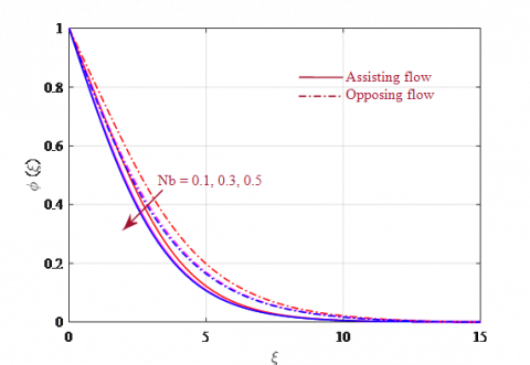
Figure 17. Graph for concentration distribution for various values of Nb
Figure 13,14,15,16,17 and 18 depicts nanoparticles concentration $\phi(\xi)$ distribution with increasing of PowellEyring fliud parameter $\varepsilon$, thermal buoyancy $\beta,$ mass buoyancy $\delta,$ thermophoresis parameter $N t,$ Brownian motion $N b$ andLewis number $L e$ for both opposing and promote flow condition. The Figure $13,$ is clear that the concentration contour increases with increase in $\mathrm{F}$ for mutual conditions. The nanoparticles concentration and solute buoyancy layer thickness are decreases for increasing $\beta$ or $\delta$ inreverse trend and assisting flow case is noticed for opposing flow is used (see Figure 14 and 15 ). Figures 16 and 17 shows that how the concentration contours differ that Brownian motion parameter $N b$ and thermophoresis parameter $N t$.
Figure 16 shows all enlarge by the concentration and the solutal buoyancy layer diameter within increasing in the thermophoresis parameter, duration of the decrease in the concentration and the solutal buoyancy layer diameter is seen in Figure 17 says that increasing rates of the Brownian motion parameter. This concentration buoyancy layer thickness decreases with increase in $L e$ for both cases which is observed in Figure $18 .$ Figure 19,20 and 21 show the validations in the skin friction coefficient, the Sherwood number and the local Nusselt number for various values of the thermophoresis and the Brownian motion. From the Figure $19,$ is noticed that the surface shear stress value decreases with increase in $N b$ in occurrence of opposing flow and opposite for aiding flow case, for aiding flow condition the surface shear stress rate decrease at increase in $N t$ it increases for opposing case.
Figure 18. Graph for concentration distribution for Le
Figure 19. Graph for skin friction coefficient for Nt and Nb for both assisting and opposing flows
Figure 20. Graph for local Nusselt number for various values of Nt and Nb for both assisting and opposing flows
From Figure 20, shows evident the Nusselt number decrease at the Brownian motion and thermophoresis for both cases. Physical reason is the pressure of the Brownian motion and thermophoresis has been tendency to increase in the thermal situation of fluid source its heat and thermal buoyancy layer thickness is increase; consequently, the temperature conducts the rate is decreases. The mass transfer valueis decreases with the increase in Nt while it is increases with increase in $N b$, this is observed in Figure 21 for both occurrences. The final result that all the contours equate the free stream boundary conditions (13) asymptotically, the guarantees accuracy of the numerical scheme.
Figure 21. Graph for local Sherwood number for various values of Nt and Nb for both assisting and opposing flows
From the present study mixed convection flow of steady non-Newtonian Powell-Eyring nanofluid over a stretching sheet under the effects of thermophoresis and Brownian motion with heat generation/absorption is analyzed. Some of the observations are listed below:
All these observations are consistent with earlier findings in the literature. Moreover, the results show that the Spectral Quasi Linearization Method is productive and sufficiently amazing for utilization of taking care of solving fluid flow problems.
[1] Imtiaz, M., Hayat, T., Hussain, M., Shehzad, S.A., Chen, G.Q., Ahmad, B. (2014). Mixed convection flow of nanofluid with Newtonian heating. The European Physical Journal, 129: 97 https://doi.org/10.1140/epjp/i2014-14097-y
[2] Akram, S., Ghafoor, A., Nadeem, S. (2012). Mixed convective heat and mass transfer on a peristaltic flow of a non-Newtonian fluid in a vertical asymmetric channel. Heat Transfer-Asian Research, 41(7): 613-633. https://doi.org/10.1002/htj.21020
[3] Mohammad, M., Ayub, G., Asghar, M.D. (2011). Mixed-convection flow of nanofluids and regular fluids in vertical porous media with viscous heating. Industrial & Engineering Chemistry Research, 50(15): 9403-9414. https://doi.org/10.1021/ie2003895
[4] Choi, S.U.S. (1995). Enhancing thermal conductivity of fluids with nanoparticles. Development and Applications of non-Newtonian Flows, Siginer D.A. and Wang HP, eds, ASME MD- 231, 66: 99-105.
[5] Xuan, Y., Roetzel, W. (2000). Conceptions for heat transfer correlation of nanofluids. Int J Heat Mass Trans, 43(19): 3701-3707. https://doi.org/10.1016/S0017-9310(99)00369-5
[6] Khanafer, K., Vafai, K., Lightstone M. (2003). Buoyancy-driven heat transfer enhancement in a two-dimensional enclosure utilizing nanofluids. International Journal of Heat and Mass Transfer, 46(19): 3639-3653. https://doi.org/10.1016/S0017-9310(03)00156-X
[7] Nadeem, S., Ul Haq, R., Akbar, N.S., Lee, C., Khan, Z.H. (2013). Numerical study of boundary layer flow and heat transfer of Oldroyd-B nanofluid towards a stretching sheet. PLoS ONE, 8(8): e69811. https://doi.org/10.1371/journal.pone.0069811
[8] Nadeem, S., Lee C. (2012). Boundary layer flow of nanofluid over an exponentially stretching surface. Nanoscale Research Letters, 7: 94. https://doi.org/10.1186/1556-276X-7-94
[9] Tan, W.C., Masuoka, T. (2005). Stokes problem for a second-grade fluid in a porous half space with heated boundary. International Journal of Non-Linear Mechanics, 40(4): 515-522. https://doi.org/10.1016/j.ijnonlinmec.2004.07.016
[10] Fetecau, C., Zierep, J., Bohning, R., Fetecauc, C. (2010). On the energetic balance for the flow of an Oldroyd-B fluid due to a flat plate subject to a time-dependent shear stress. Computers & Mathematics with Applications, 60(1): 74-82. https://doi.org/10.1016/j.camwa.2010.04.031
[11] Hayat, T., Abbas, Z., Pop, I., Asghar, S. (2010). Effects of radiation and magnetic field on the mixed convection stagnation-point flow over a vertical stretching sheet in a porous medium. International Journal of Heat and Mass Transfer, 53(1-3): 466-474. https://doi.org/10.1016/j.ijheatmasstransfer.2009.09.010
[12] Ishak, A., Nazar, R., Amin, N., Filip, D., Pop I. (2007). Mixed convection of the stagnation-point flow towards a stretching vertical permeable sheet. Malaysian Journal of Mathematical Sciences, 2: 217-226.
[13] Powell, R.E., Eyring, H. (1944). Mechanism for relaxation theory of viscosity. Nature, 154: 427-428. https://doi.org/10.1038/154427a0
[14] Satyaban, P., Motahar, R., Akshya Kumar, M. (2015). Mixed convective flow of a powell-eyring fluid over a non-linear stretching surface with thermal diffusion and diffusion thermo. International Conference on Computational Heat and Mass Transfer-2015. Procedia Engineering, 127: 645-651. https://doi.org/10.1016/j.proeng.2015.11.356
[15] Malik, M.Y., Khan, I., Hussain, A., Salahuddin, T. (2015). Mixed convection flow of MHD Eyring-Powell nanofluid over a stretching sheet: A numerical study. AIP Advances, 5: 117118. https://doi.org/10.1063/1.4935639
[16] Javed, T., Ali, N., Abbas, Z., Sajid, M. (2013). Flow of an Eyring -Powell non- Newtonian fluid over a stretching sheet. Chemical Engineering Communications, 200(3): 327-336. https://doi.org/10.1080/00986445.2012.703151
[17] Nadeem, S., Hayat, T., Abbas, S., Ali, M. (2010). Effects of partial slip on a fourth- grade fluid with variable viscosity: An analytic solution, nonlinear analysis. Real World Applications, 11(2): 856-868. https://doi.org/10.1016/j.nonrwa.2009.01.030
[18] Ishak, A., Nazar, R., Pop, I. (2008). Mixed convection stagnation point flow of a micropolar fluid towards a stretching sheet. Meccanica, 43: 411-418. https://doi.org/10.1007/s11012-007-9103
[19] Gangadhar, K., Keziya, K., Ibrahim, S.M. (2019). Effect of thermal radiation on engine oil nanofluid flow over a permeable wedge under convective heating: Keller box method. Multidiscipline Modeling in Materials and Structures, 15(1): 187-205. https://doi.org/10.1108/MMMS-03-2018-0047
[20] Gangadhar, K., Sobhana Babu, P.R., Venkata Subba Rao, M. (2018). Microstructure and inertial characteristic of a magnetite Ferro fluid over a stretched sheet embedded in a porous medium with viscous dissipation using the spectral quasi-linearisation method. International Journal of Ambient Energy. https://doi.org/10.1080/01430750.2018.1563823
[21] Gangadhar, K., Kannan, T., DasaradhaRamaiah, K., Sakthivel, G. (2018). Boundary layer flow nanofluids to analyse the heat absorption/generation over a stretching sheet with variable suction/injection in the presence of viscous dissipation. International Journal of Ambient Energy. https://doi.org/10.1080/01430750.2018.1501738
[22] Gangadhar, K., Kannan, T., Sakthivel, G., Dasaradha Ramaiah, K. (2018). Unsteady free convective boundary layer flow of a nanofluid past a stretching surface using a spectral relaxation method. International Journal of Ambient Energy. https://doi.org/10.1080/01430750.2018.1472648
[23] Gangadhar, K., Kannan, T., Jayalakshmi, P. (2018). MHD micropolar nanofluid past a permeable stretching/shrinking sheet with Newtonian heating. Journal of the Brazilian Society of Mechanical Sciences and Engineering, 39(11): 439-4391.
[24] Venkata Subba Rao, M., Gangadhar, K., Varma, P.L.N. (2018). A spectral relaxation method for three-dimensional MHD flow of nanofluid flow over an exponentially stretching sheet due to convective heating: An application to solar energy. Indian Journal of Physics, 92(12): 1577-1588. https://doi.org/10.1007/s12648-018-1226-0
[25] Bellman, R.E., Kalaba, R.E. (1965). Quasi linearization and Non-Linear Boundary-Value Problems. American Elsevier Publishing Company, New York.
[26] Canuto, C., Hussaini, M.V., Quarteroni, A., Zang, T.A. (1988). Spectral Methods in Fluid Dynamics. Springer, Berlin.
[27] Rashidi, M.M., Vishnu Ganesh, N., Abdul Hakeem, A.K., Gangad, B. (2014). Buoyancy effect on MHD flow of nanofluid over a stretching sheet in the presence of thermal radiation. Journal of Molecular Liquids, 198: 234-238. https://doi.org/10.1016/j.molliq.2014.06.037
[28] Wang, C.Y. (1989). Free convection on a vertical stretching surface. Journal of Applied Mathematics and Mechanics (ZAMM), 69: 418-420. https://doi.org/10.1002/zamm.19890691115