Mohammad Reza Salehizadeh* | Hassan Nouri
© 2020 IIETA. This article is published by IIETA and is licensed under the CC BY 4.0 license (http://creativecommons.org/licenses/by/4.0/).
OPEN ACCESS
Circuit theory is a cornerstone course in electrical engineering and control majors in ordinary universities and colleges throughout the world. This course covers fundamental principles and analysis methods of basic circuits commonly employed in the forthcoming courses. In most electrical programs after the introduction of basic elements of Ohm’s and Kirchhoff’s current and voltage laws, the dynamic response of the circuits containing capacitors and inductors will be studied. Customarily to solve these circuits, advanced mathematical approaches such as differential equations are used. Under such circumstances, the students are faced with two challenges, solving the differential equations, and understanding the dynamic response of circuits. In order to improve students’ understanding, an analysis tool with less mathematical prerequisites should be used for the solutions before embarking on the use of conventional differential equation techniques such as Laplace transform. Hence, we propose a novel approach for these circuit analyses through the application of a discretized version of differential equations which is used in discrete control systems. Although this approach has a well-established background, its exploration uses in the circuit theory course as yet has not been reported. The novelty of the proposed approach not only lies in its intuitive simplicity but also in its contribution to the understanding and visualization of students in the real-time response of linear and non-linear circuits to any desirable input without any mathematical burden. The analysis can be performed by hand or this is also helpful for those who prefer modern education aided by computers. This, in turn, may attract more students to the program. In this paper, the effectiveness of the proposed approach is demonstrated through a set of illustrative examples.
circuit, modelling, difference equation, dynamic response, non-linear circuits
According to the U.S. Bureau of Labor Statistics, Employment Projections program, the employment of electrical engineers is projected to grow 7 percent from 2016 to 2026 [1]. Taking any step towards improvement of the content and teaching style of the fundamental courses in electrical engineering programs will enhance the scientific background of these new generation of engineers. Without doubt, circuit theory is one of the most important and fundamental courses in the electrical engineering curriculum throughout the world [2, 3]. Rather than electrical engineering major, learning and research in a few other majors such as automation, and computer science is based on circuit theory [4]. Specifically, in electrical engineering, the knowledge acquired in this course is a prerequisite for most of the advanced courses such as electronics, power system analysis, and electrical machines. Given this introduction about the importance of circuit analysis course, many researches have been devoted to the success of the students in this course [5]. These approaches include, but not limited to, improving teaching style [6, 7], text book selection [8], and improving teaching materials [9]. Despite of these researches, further steps need to be taken to fulfill the gaps in the content of this important course. This paper intends to address this important issue by proposing incorporation of circuit analysis through difference equation in the content of circuit analysis course.
In circuit theory course, after the introduction of R, L, C combination, ohm’s law, and Thevenin’s theorem, the students are familiarized with the analysis of first and second order transient response of a circuit [10]. In this regard, the basic definitions, concepts, theorems, and tools for analysis of a circuit are instructed. To this purpose, acquiring fundamental knowledge of physics, including the basics of electricity and magnetism, and mathematics, including knowledge of solving algebraic and differential equations, are the prerequisite for this course. Most of the students who participate in this course have knowledge of basic algebraic equations from high school. However, the students usually become familiar with differential equations through university courses. Having the knowledge to solve differential equations is necessary in some parts of the circuit theory course such as analysis of RLC circuits. According to the information gathered from Iranian and some European instructors, in spite of having a background in differential equations, most students who take a circuit theory course do not have sufficient mastery in solving these equations. Under such cases, instructing dynamic analysis of the circuits faces some challenges. Due to the lack of essential mastery on differential equation solution methods, the students are not able to fully focus on the analysis of such circuits. This in turn may lead to decreased motivation and attraction to this course. To overcome these challenges, regardless of the students’ competence to solve differential equations, a soft start topic with less mathematical requirements needs to be introduced as an extension to this course before embarking on solving directly the differential equation. With this aim, we propose to initially familiarize students with the conversion method of differential equations to difference equations by a discretization process. Thereafter, to analyze the obtained difference equations either by hand or by writing simple codes. In general, the proposed has a number of benefits including increased appeal of circuit theory to students’ and provision of more time for students to focus on the concept and engineering analysis of the circuit without facing mathematical challenges at the beginning of the course. This enhances their competence in the solution of differential equations, understanding real-time response of an electrical circuit to any desirable input, and finally enabling them to produce simple codes to understand non-linear circuits without any mathematical burden. Although the modeling and analysis of dynamic systems through difference equations has a very established background, from an educational perspective the proposed approach is novel. To date no report can be found in published educational literature where differential equations represent the circuit model transformed into the difference equations in circuit theory course.
The remainder of the paper is organized as follows; section II discusses in brief the review on difference equations. A set of illustrative examples are solved in section III where also the advantages of the proposed approach is demonstrated. Section IV concludes the paper.
2.1 Difference equation
In simple words, a mathematical equation with a function and its related derivatives is called a “differential equation”. A differential equation is usually used to model continuous dynamic systems. In contrary, difference equation consists of the differences between successive values of a function of a discrete variable. Two well-known mathematical transforms, Laplace and z-transform, are used to find the close-form solution for differential and difference equations, respectively. Solving a differential equation yields the analog signal, while solving difference equations yields digital signals. Difference equations are used to model discrete dynamic control systems or to approximate continuous dynamic systems. Approximation of differential equations by difference equations is useful for cases in which a close-form solution is not possible to be obtained for differential equations. For an instant, consider a dynamic system that is presented with the following mathematical model: $y^{\prime}(t)+y(t)=\sin (t) .$ From the definition of the derivative, we have $y^{\prime}(t) \cong \frac{y(t+\Delta t)-y(t)}{\Delta t}$ where $\Delta t$ should be chosen as small as possible. By defining $t=k \Delta t$ in which $k=0,1,2, \ldots,$ we have $y(t)=y(k)$ $y^{\prime}(t) \cong \frac{y(k+1)-y(k)}{\Delta t},$ and $\sin (t)=\sin (k) .$ The equivalent difference equation would be $\frac{y(k+1)-y(k)}{\Delta t}+y(k)=$ $\sin (k), k=0,1,2, \ldots .$ The smaller value for $\Delta t$ results in a more precise approximation. This approximation can be employed for both linear and non-linear differential equations. Given the initial condition, the resultant difference equation can be implemented through a computer code. This approach for solving differential equations becomes important, especially when we face non-linearity. This approach has been used extensively for solving engineering problems. For example, to design an optimal control method by means of a dynamic programming approach, the differential equations need to be approximated by difference equations [11]. An application for computer control of practical continuous-time processes is proposed by Yang and Ding [12]. Dynamic behaviors of nonlinear models arising in ocean engineering are treated through a similar way [13]. As shown in these papers [5, 6] in the engineering practice approximation by difference equation is used for solving non-linear and complicated systems. However, as stated in the introduction, from an educational perspective, not only for the analysis of nonlinear circuits, but also for linear circuits, establishing an additional course based on difference equation has some merits.
2.2 Step-by-step procedure
The proposed procedure of the educational course is as follows:
i) Instruction of modeling dynamic circuits: At this step by using KVL and KCL laws, the set of differential equations is derived.
ii) Instruction of discretization: The obtained differential equations from the previous step is discretized in the following form:
$\theta(k+1)=A \theta(k)+B u(k) \quad k=0,1, \ldots, N$ (1)
where, θ is the state vector that could be voltage or current and u is the input of the circuit. It is noticed that θ are n×1 vector in which n is the order of the circuit.
iii) Instruction of what happens to the instantaneous voltages and currents which have been discretized and shown as the state vector (θ). With this aim, the following pseudocode could be used to solve the recursive equation of (1).
|
Begin |
|
Input A, B, θ(0) |
|
Do |
|
Repeat k=0:N |
|
θ(k+1)=Aθ(k)+Bu(k) |
|
End |
iv) Asking the students to develop codes for some of the relevant exercises to obtain a better level of understanding.
In this section, we will provide three simple educational examples to show the advantages of the proposed approach.
3.1 Linear-time invariant circuit
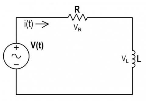
The schematic of RL circuit is shown in Figure 1.
Figure 1. A simple RL circuit
Following the step-by-step procedure of II-B, the dynamic equation for this circuit is formed by Kirchhoff’s voltage law (KVL):
$R i(t)+L \frac{d i(t)}{d t}=V(t)$ (2)
The differential equation is transformed to a difference equation. Dividing the time interval $[0, t]$ into $N$ increments of $\Delta t,$ yields $t=k \Delta t,$ in which $k=0,1, \ldots, N .$ The resultant difference equation becomes:
$R i(k)+L \frac{i(k+1)-i(k)}{\Delta t}=V(k)$
(k=0,1,…,N) (3)
The re-arrangement of (3) is:
$i(k+1)=\left(1-\frac{R \Delta t}{L}\right) i(k)+\frac{\Delta t}{L} V(k)$ (4)
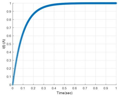
Considering $R=1 \Omega, L=0.1 H, \Delta t=0.001$ second, $t=1 second, and the input is a step function $(V(t)=u(t)),$ Eq. $\begin{array}{lllll}\text { (4) } & \text { yields } & \text { as } & i(k+1)=0.98 i(k)+0.01 u(k) & . & \text { This }\end{array}$ difference equation is solved using the pseudocode of section II. The students can also solve this equation by hand. At $t=0$ second, considering $k=0, u(0)=1$ and the initial current $i(0)=0,$ then $i(1)=0.01 .$ Similarly at $t=1$ second, $k=1$ $u(1)=1$ and $i(1)=0.01,$ then $i(2)=0.0198,$ and so on. As it is observed the students are able to easily follow what is happening in real-time simulation and how the instantaneous values of the input voltage and currents affect the result. Such observation and analysis are not easily possible via direct solution of the differential equation. Additionally, the students can easily code this procedure in any programming device or software. As an example the following code is written for MATLAB environment that is related to the problem of Figure 1. Its corresponding result is shown in Figure 2.
clear all; clc; close all
|
R=1; L=0.1; |
|
dt=1e-3; |
|
t=0:dt:1; |
|
y=[0]; |
|
for k=1:length(t)-1 |
|
y(k+1)=(1-R*dt/L)*y(k)+dt*1/L; |
|
end |
|
plot(t,y,'*') |
The same result can be obtained through direct solution of conventional differential equations [3].
Figure 2. Current of a simple RL circuit resultant from difference equation
3.2 Non-linear-time invariant circuit
To show the effectiveness of the proposed methodology for instruction of non-linear circuits, assume that the inductance of the circuits shown in Figure 1 is now nonlinear that has the flux linkage of:
$\mathrm{i}(\lambda)=95 \lambda^{5}+\frac{100 \lambda^{3}}{\lambda+5}+\lambda$.
Applying KVL results the following nonlinear differential equation:
$\frac{d \lambda}{d t}+95 \lambda^{5}+\frac{100 \lambda^{3}}{\lambda+5}+\lambda=u(t)$ (5)
This type of example is not expected to be solved by students who are taking this course. However, here it is solely used as an educational example. Analysis of such an example could easily be understood via the proposed procedure in which the discretization of Eq. (5) results in the following difference equation:
$\lambda(k+1)=-0.095 \lambda^{5}(k)+0.999 \lambda(k)-\frac{0.1 \lambda^{3}(k)}{\lambda(k)+5}$
$+0.001 u(k) \leftrightarrow$ (6)
The solution for the Eq. (6) is similar to the earlier example in which at $t=0$ second, $k=0, u(0)=1$ and $\lambda(0)=0,$ then $\lambda(1)=0.001 .$ Also at $t=1$ second, $k=1, u(1)=1$ and $\lambda(1)=0.001,$ then $\lambda(2)=0.002$ as shown below: $\lambda(2)=$ $-0.095(0.001)^{5}+0.999(0.001)+\frac{0.1(0.001)^{3}}{(0.001)+5}+0.001=$ $0.002 .$ and so on. The MATLAB code for this problem is illustrated below.
|
clear all;clc; close all |
|
dt=1e-3; |
|
t=0:dt:1; |
|
lambda=[0]; |
|
i=[0]; |
|
for k=1:length(t)-1 |
|
lambda(k+1)=-.095*lambda(k)^5+0.999*lambda(k)-.1*lambda(k)^3/(lambda(k)+5)+.001; |
|
i(k+1)=95*lambda(k+1)^5+100*lambda(k)^3/(lambda(k)+5)+lambda(k); |
|
end |
|
plot(t,lambda,'*') |
|
ylabel('\lambda(Wb)') |
|
xlabel('Time(sec)') |
|
plot(t,i,'*') |
|
ylabel('i(A)') |
|
xlabel('Time(sec)') |
Figures 3 and 4 show the magnetic flux of the nonlinear inductance and current of the circuit, respectively.
Figure 3. RLC circuit without external resources
Figure 4. Current of the inductor in RLC circuit
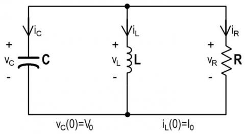
3.3 Second order R-L-C circuit
The proposed educational approach is able to be applied to higher order circuits. To show this capability, an RLC circuit without external resources is considered as shown in Figure 3. By applying KCL the following state-space equations will be derived for this circuit:
$\left[\begin{array}{c}\frac{d i_{L}}{d t} \\ \frac{d V_{c}}{d t}\end{array}\right]=\left[\begin{array}{cc}0 & \frac{1}{L} \\ \frac{-1}{C} & \frac{-1}{R C}\end{array}\right]\left[\begin{array}{c}i_{L} \\ V_{c}\end{array}\right]$ (7)
Discretizing these equations yields
$\left[\begin{array}{c}i_{L}(k+1) \\ V_{c}(k+1)\end{array}\right]=\left[\begin{array}{cc}1 & \frac{\Delta t}{L} \\ \frac{-\Delta t}{C} & 1-\frac{\Delta t}{R C}\end{array}\right]\left[\begin{array}{c}i_{L}(k) \\ V_{c}(k)\end{array}\right]$ (8)
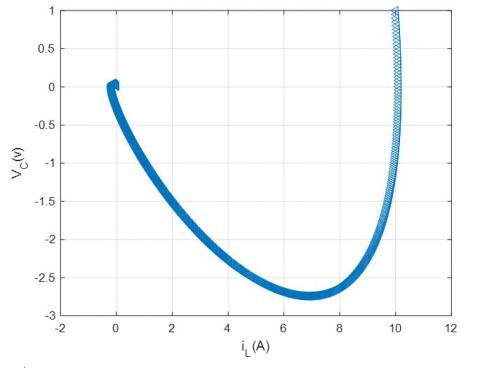
By setting the initial condition and parameters as $i_{L}(0)=$ $0, V_{C}(0)=0, R=1 \Omega, L=0.1 H, C=0.001 F, \Delta t=$ 0.001 second and $t=1$ second. The inductance current, capacitor voltage, and the state trajectory are obtained and shown in Figures $4-6, $ respectively.
Figure 5. Current of the inductor in RLC circuit
Figure 6. State trajectory of RLC circuit
In this paper, we proposed circuit analysis through difference equations which is frequently used in discrete control approaches. The novelty and effectiveness of the proposed approach have been demonstrated. The approach is simple and complementary for the teaching of a typical circuit analysis course before embarking on the use of differential equation approach. Furthermore, the proposed approach has a number of benefits including increased student attraction to circuit theory and provision of more time for students to focus on the concept and engineering analysis of circuits without facing mathematical challenges at the earlier stage of the course. This will enhance their competence in the solution of differential equations, their understanding of real-time response of an electrical circuit to any desirable input, and will enable them to produce simple codes to understand linear and non-linear circuits without any mathematical burden such as Laplace Transform. Also, the approach could be applied to any circuit with any order. Moreover, as shown in the developed codes, the used commands are very basic and simple and a student who has passed a basic programming course will be able to write such codes by any programming package without the need for in-depth mathematical knowledge. The developed educational course could be applied in other engineering disciplines for which the dynamics of the systems need to be instructed. For instance, vibration theory course in mechanical engineering, and introduction to heat transfer course in chemical engineering.
[1] Bureau of Labor Statistics, U.S. Department of Labor. (2020). Occupational Outlook Handbook, Electrical and Electronics Engineers. https://www.bls.gov/ooh/architecture-and-engineering/electrical-and-electronics-engineers.htm, accessed on October 12, 2019.
[2] Kirk, D.E. (2004). Optimal Control Theory: An Introduction. Courier Corporation.
[3] Desoer, C.A. (2010). Basic Circuit Theory. Tata McGraw-Hill Education.
[4] Xu, J.Q., Li, K.N., Liang, Q.F. (2018). Practice and research on the reform of teaching methods in circuit course. In 2018 International Seminar on Education Research and Social Science (ISERSS 2018), Atlantis Press. https://doi.org/10.2991/iserss-18.2018.38
[5] Parent, D.W. (2018). Examination the impact of various factors on student success in an introduction to circuit analysis course. In 2018 IEEE Frontiers in Education Conference (FIE), San Jose, CA, USA, pp. 1-5. https://doi.org/10.1109/FIE.2018.8659259
[6] Hoic-Bozic, N., Mornar, V., Boticki, I. (2008). A blended learning approach to course design and implementation. IEEE Transactions on Education, 52(1): 19-30.
[7] Liu, Z., Zhao, W.Y., Xie, H., Zhong, H.S., Cui, H.L. (2018). Research of a multi-element teaching method in retaking course of circuit analysis. Journal of Electrical & Electronic Education, 2: 31.
[8] Sangam, D., Jesiek, B K. (2014). Conceptual gaps in circuits textbooks: A comparative study. IEEE Transactions on Education, 58(3): 194-202. https://doi.org/10.1109/TE.2014.2358575
[9] Johnson, A.M., Butcher, K.R., Ozogul, G., Reisslein, M. (2013). Introductory circuit analysis learning from abstract and contextualized circuit representations: Effects of diagram labels. IEEE Transactions on Education, 57(3): 160-168. https://doi.org/10.1109/TE.2013.2284258
[10] Parent, D.W. (2017). Novel gateway stay/add policy used to increase student success rates in an introductory circuits class. In 2017 IEEE Frontiers in Education Conference (FIE), Indianapolis, IN, USA, pp. 1-8. https://doi.org/10.1109/FIE.2017.8190600
[11] Ge, Y., Li, S., Chang, P. (2018). An approximate dynamic programming method for the optimal control of Alkai-Surfactant-Polymer flooding. Journal of Process Control, 64: 15-26. https://doi.org/10.1016/j.jprocont.2018.01.010
[12] Yang, D., Ding, R. (2014). Transforms from differential equations to difference equations and vice-versa applied to computer control systems. Applied Mathematics Letters, 31: 18-24. https://doi.org/10.1016/j.aml.2013.12.011
[13] Sulaiman, T., Bulut, H., Yokus, A., Baskonus, H. (2019). On the exact and numerical solutions to the coupled Boussinesq equation arising in ocean engineering. Indian Journal of Physics, 93(5): 647-656. https://doi.org/10.1007/s12648-018-1322-1