Cheekolu Murali Krishna | Gottam Viswanathan Reddy | Surapuraju Suresh Kumar Raju | Chakravarthula Siva Krishnam Raju | Fazle Mabood*
© 2020 IIETA. This article is published by IIETA and is licensed under the CC BY 4.0 license (http://creativecommons.org/licenses/by/4.0/).
OPEN ACCESS
This communication explores natural convection of magnetohydrodynamic Blasius and Sakiadis fluid flows with active and passive controls of nanoparticles. The Brownian and thermophoresis effects are added to energy equation. Chemically reactive species are taken into account for first-order and higher-order chemical reactions. The similarity transformation technique is employed to translate the governing partial differential equations into ordinary differential equations and then solved with R-K method with shooting technique. How the velocity, temperature and concentration distributions are effected by distinct physical flow parameters are analyzed and sketched graphically. Skin friction coefficient, local Nusselt and Sherwood numbers are also computed and analyzed with passive and active flows for both Blasius and Sakiadis fluid flows. We found that the Biot number due to thermal enhances the rate of heat transfer rate in active and passive flows for both Sakiadis and Blasius fluid flows.
Blasius flow, Sakiadis flow, chemical reaction, active and passive flows
The nanofluids have a numerous applications and usages in different branches of science and technology like medicine, automobiles, fabrication and food processing. The nanoparticles are homogeneously diffused in the base fluid; resultantly fluid thermal properties are enhanced. The active and passive control of nanoparticles is also playing a major portion in nanofluids. Ibrahim [1] presented a passive control of nanoparticles in second order slip flow of micropolar fluid over a stretching sheet with convective boundary condition and he noted that the concentration graph tends to zero far away from the sheet. Tripathi et al. [2] simultaneously investigated the viscous dissipation and hall current effects on three-dimensional flow of hydromagnetic nanofluid in horizontal rotating channel in presence of active and passive control of nanoparticles and they noted that the volume fraction has negative value at the lower plate with passive control of nanoparticles. Acharya [3] proposed a fabrication of passive and active controls of nanoparticles on stagnation point flow of an unsteady nanofluid and they concluded that temperature is always found to increase in active model as compared to passive model. Hayat et al. [4] investigated the conducting flow of Jeffery nanofluid with active and passive controls of nanoparticles over a non-linear stretching sheet. They stated that the specious concentration reduced with Brownian motion parameter in both active and passive cases. The stagnation point flow of Maxwell nanofluid over a slipped stretched surface with passive and active control of nanoparticles is considered by Halim et al. [5] and they stated that the stagnation parameter promotes heat transformation of the flow under passive and active controls of nanoparticles. Halim et al. [6] presented the passive and active control of nanoparticles on steady incompressible stagnation point flow of Williamson nanofluid across a horizontal linear stretching or shrinking sheet and they stated that the effect of Lewis number is negligible in heat transfer rate on passive control case. Wagner et al. [7] discussed the segmentation and classification of Nanoparticle Diffusion trajectories in cellular micro environments. Muhammad et al. [8] presented the boundary layer flow of hydromagnetic Maxwell nanofluid over a stretching sheet saturating a non-Darcy porous medium and they found that the rate of heat transfer is lower at the plate for large values of thermophoresis parameter.
The heat transfer analysis is also an important thing in nanofluid flows with Sakiadis and Blasius flow models. The following are the few investigations on Blasius and Sakiadis flows with various modes of heat transfer. The velocity and temperature distributions on thermal boundary layer over a semi-infinite flat plate were presented by Kuo [9]. Hossain et al. [10] investigated the thermal radiation effect on natural convection flow over heated vertical porous plate and they noticed that the viscosity parameter and radiation parameter are significant in local Nusselt number and local skin friction. Rapits et al. [11] studied the effect of thermal radiation on conducting flow over a semi-infinite stationary plate. Bataller [12] discussed the convective boundary condition on Blasius and Sakiadis flows with thermal radiation effect and he concluded that the Sakiadis flow provides a thinner thermal boundary layer compared with the Blasius flow. Fang et al. [13] presented a heat transfer on generalized shrinking or stretching wall and they observed a higher dropping slope with higher values of Prandtl number. Garg et al. [14] evaluated the problem of thermal boundary layer on stationary flat plate in a uniform stream of fluid with convective boundary condition and they concluded that the fluid temperature increases with Biot number in the case of without internal heat generation. An unsteady convective boundary layer viscous fluid flow over a vertical stretching surface with thermal radiation and variable transport properties were presented by Vajravelu et al. [15] and they stated that there exists a thicker thermal boundary layer in suction case compared to impermeability. We found a novel literature about heat transformation over a boundary layer flows with various flow conditions in references [16-26].
Stimulation of above discussed applications and investigations, in this current study we presented the active and passive controls of nanoparticles on natural convection of electrically conducting fluids in Sakiadis and Blasius flow cases with chemical reaction. We presented and discussed the velocity, temperature and concentration distributions in graphically in active and passive control cases in both Blasius and Sakiadis flow cases. Moreover local skin friction coefficients, heat and mass transformations at the surface are represented numerically in Blasius and Sakiadis flow cases through tables.
Consider an unsteady natural convection of Blasius and Sakiadis magnetohydrodynamic flows with variable properties (viscosity and thermal conductivity) and porous layers. To control thermal and concentration boundary layers we also considered the combined effect of Brownian motion and thermophoresis as well as viscous dissipation and thermal radiation with active and passive control of nanomaterial’s conditions. It coincides with the y=0 (Figure 1).
Figure 1. The physical model of the flow configuration
The Cartesian coordinate system has its origin located at the leading edge with the positive x-axis extending along the sheet in the upwards direction, while the y-axis is measured normal to the flow. We assume that for time t <0 the fluid. The unsteady fluid heat flows start at t = 0, the sheet is being stretched with the velocity $U_{w}(x, t)=\frac{a x}{1-c t}$ along the x-axis, keeping the origin fixed. The thermo-physical properties of the sheet or plate and the ambient fluid are assumed to be constant except density variations and the thermal conductivity which are assumed to vary linearly with temperature. The assumptions (with the Bossiness and boundary layer approximations) are, the governing equations for the convective flow and heat and mass transfer of the viscous fluid [20-24] are:
$\frac{\partial u}{\partial x}+\frac{\partial v}{\partial y}=0$, (1)
$\frac{\partial u}{\partial t}+u \frac{\partial u}{\partial x}+v \frac{\partial u}{\partial y}=\frac{1}{\rho} \frac{\partial}{\partial y}\left(\mu_{f} \frac{\partial u}{\partial y}\right)+$
$g\left(\beta_{c}\left(C-C_{\infty}\right)+\beta_{T}\left(T-T_{\infty}\right)\right)-\frac{\sigma B_{0}^{2}}{\rho} u-\frac{\vartheta}{K_{0}} u$ (2)
$\rho C_{p}\left(\frac{\partial T}{\partial t}+u \frac{\partial T}{\partial x}+v \frac{\partial T}{\partial y}\right)=\frac{\partial}{\partial y}\left(K(T) \frac{\partial T}{\partial y}\right)+$
$\mu_{f}\left(\frac{\partial u}{\partial y}\right)^{2}+\tau\left(\begin{array}{c}D_{B} \frac{\partial T}{\partial y} \frac{\partial C}{\partial y} \\ +\frac{D_{T}}{T_{\infty}}\left(\frac{\partial T}{\partial y}\right)^{2}\end{array}\right)+\frac{16 \sigma^{*} T_{\infty}^{3}}{3 k^{*}} \frac{\partial^{2} T}{\partial y^{2}}$ (3)
$\frac{\partial C}{\partial t}+u \frac{\partial C}{\partial x}+v \frac{\partial C}{\partial y}=D_{B} \frac{\partial^{2} C}{\partial y^{2}}-k_{0}\left(C-C_{\infty}\right)^{n}+$
$\frac{D_{T}}{T_{\infty}} \frac{\partial^{2} T}{\partial y^{2}}$ (4)
Subject to the boundary conditions are:
Passive control of nanomaterials:
$\left.\begin{array}{l}v=0, u=0, k_{\infty} \frac{\partial T}{\partial y}=-h_{f_{1}}\left(T-T_{\infty}\right) \\ D_{B} \frac{\partial C}{\partial y}+\frac{D_{T}}{T_{\infty}} \frac{\partial T}{\partial y}=0, a t y=0 \\ u=U_{w}, T=T_{\infty}, C=C_{\infty} \text { as } y \rightarrow \infty\end{array}\right\}$ (5)
$\left. \begin{align} & v=0,\,u={{U}_{w}},{{k}_{\infty }}\frac{\partial T}{\partial y}=-{{h}_{{{f}_{1}}}}(T-{{T}_{\infty }}), \\ & {{D}_{B}}\frac{\partial C}{\partial y}+\frac{{{D}_{T}}}{{{T}_{\infty }}}\frac{\partial T}{\partial y}=0,\,at\,y=0, \\ & u=0,T={{T}_{\infty }},C={{C}_{\infty }}\,\,as\,\,y\to \infty \\ \end{align} \right\}$ (6)
The active control of nanomaterial
$\left.\begin{array}{l}v=0, u=0, k_{\infty} \frac{\partial T}{\partial y}=-h_{f_{1}}\left(T-T_{\infty}\right), \\ C=C_{w} \text { at } y=0, \\ u=U_{w}, T=T_{\infty}, C=C_{\infty} \text { as } y \rightarrow \infty\end{array}\right\}$ (7)
$\left. \begin{align} & v=0,\,u={{U}_{w}},{{k}_{\infty }}\frac{\partial T}{\partial y}=-{{h}_{{{f}_{1}}}}(T-{{T}_{\infty }}), \\ & C={{C}_{w}}\,at\,y=0, \\ & u=0,T={{T}_{\infty }},C={{C}_{\infty }}\,\,as\,\,y\to \infty \\ \end{align} \right\}$ (8)
Here $u$ and $v$ are the velocity components in the $x$ and $y$ directions, respectively, $v$ is the kinematic viscosity, $g$ is the acceleration due to gravity, $\beta_{T}, \beta_{C}$ is the coefficient of thermal and concentration expansions, $T$ is the fluid temperature, $T_{\infty}, C_{\infty}$ is the ambient temperature and concentration, $\rho$ is the density, $c_{p}$ is the specific heat at constant pressure, $K(T)$ is the variable thermal conductivity, $k_{n}$ is the chemical reaction rate, $\sigma^{*}$ is the Boltzmann constant, $k^{*}$ is Stefan constant, $h_{f_{1}}$ are the heat transfer coefficients due to thermal. In this paper the thermal conductivity and viscosity is assumed to vary linearly with temperature as:
$K(T)=K_{\infty}\left(1+\frac{\varepsilon}{\Delta T}\left(T-T_{\infty}\right)\right)$ (9)
$\mu_{f}(T)=\frac{\mu_{\infty}}{\left(1+\omega\left(T-T_{\infty}\right)\right)}$ (10)
Here $\Delta T=(T w-T \infty), \quad T_{w}$ is the surface temperature, $\varepsilon$ and $\omega$ are small parameter known as the conductivity and viscosity variation parameters, $k_{\infty}, \mu_{\infty}$ are the thermal conductivity and viscosity of the fluid far away from the surface. These particular forms of a $U_{w}(x, t)$ and $T_{w}(x, t)$ have been chosen in order to obtain a new similarity transformation, which transforms the governing partial differential Eqns. $(2)-(4)$ into a set of coupled ordinary differential equations. Defining the following dimensionless functions $\mathrm{f}$ and $\theta,$ and the similarity variable $\zeta$ as:
$\zeta=\left(\frac{a}{v(1-c t)}\right)^{\frac{1}{2}} y, \quad \psi=\left(\frac{v a}{(1-c t)}\right)^{\frac{1}{2}} x f(\zeta)$
$\theta(\zeta)=\frac{\left(T-T_{\infty}\right)}{\left(T_{w}-T_{\infty}\right)}$ (11)
where, $\quad \psi(x, y, t)$ is a stream function defined as $(u, v)=(\partial \psi / \partial y,-\partial \psi / \partial x) .$ The Substituting Eq. (11) into Eqns. $(2)-(4)$ and making use of Eqns. (7),(8) and (9) we obtain
$\frac{1}{(1+E \theta)} f^{\prime \prime \prime}-\frac{E}{(1+E \theta)^{2}} \theta^{\prime} f^{\prime \prime}+f f^{\prime \prime}-f^{\prime 2}-$
$A\left(f^{\prime}+\frac{1}{2} \zeta f^{\prime \prime}\right)+\lambda_{T} \theta+\lambda_{c} \phi-(M+K) f^{\prime}=0$ (12)
$\frac{A}{2} \zeta \theta^{\prime}-f \theta^{\prime}-\frac{1}{\operatorname{Pr}}\left(\theta^{\prime \prime}+\frac{\varepsilon}{1+\varepsilon \theta} \theta^{\prime 2}\right)-N b \theta^{\prime} \phi^{\prime}$
$-N t \theta^{\prime 2}-E c f^{\prime \prime 2}-\frac{1}{\operatorname{Pr}} \operatorname{Nr} \theta^{\prime \prime}=0$ (13)
$\frac{A}{2} \phi^{\prime} \zeta-f \phi^{\prime}=\frac{1}{L e}\left(\phi^{\prime \prime}+\frac{N t}{N b} \theta^{\prime \prime}\right)-K r \phi^{n}$ (14)
The boundary conditions are
$f(0)=0, f^{\prime}(0)=0, N b \phi^{\prime}(0)+N t \theta^{\prime}(0)=0$
$\theta^{\prime}(0)=-\left(1-B i_{1} \theta(0)\right)$
$\phi(0)=1, f^{\prime}(\infty)=1, \theta(\infty)=0, \phi(\infty)=0$ (15)
$f(0)=0, f^{\prime}(0)=1, N b \phi^{\prime}(0)+N t \theta^{\prime}(0)=0$
$\theta^{\prime}(0)=-\left(1-B i_{1} \theta(0)\right)$
$\phi(0)=1, f^{\prime}(\infty)=0, \theta(\infty)=0, \phi(\infty)=0$ (16)
where, a prime denotes differentiation with respect to $\zeta A$ $=c / a$ is that unsteady parameter, $E=\frac{\omega}{\left(T_{w}-T_{\infty}\right)}$ is viscosity variation parameter, $M=\frac{\sigma B_{0}^{2}(1-c t)}{\rho a}$ is the magnetic field parameter, $K=\frac{v(1-c t)}{k_{0} a}$ is the porosity parameter, $E c=$ $\frac{U_{w}^{2}}{c_{p}\left(T_{\infty}-T_{r}\right)},$ is Eckert number, $U_{w}^{2}=\left(\frac{a x}{1-c t}\right)^{2}, \quad N r=\frac{16 \sigma^{*} T_{\infty}^{3}}{3 k^{*} K}$ is thermal radiation, $\mathrm{Pr}=v / \alpha_{\infty}$ is the Prandtl number, $B i_{1}=$ $\frac{h_{f_{1}}}{k_{\infty}} \sqrt{\frac{v(1-c t)}{a c}}$ is thermal Biot number, $\lambda_{T}=\frac{g \beta_{T}\left(T_{w}-T_{\infty}\right)(1-c t)^{2}}{a^{2} x}$ is a thermal buoyancy, $\lambda_{C}=\frac{g \beta_{c}\left(c_{w}-c_{\infty}\right)(1-c t)^{2}}{a^{2} x},$ is concentration buoyancy, $N b=\frac{\tau D_{B}}{v \rho C_{p}}\left(C_{w}-C_{\infty}\right), N t=\frac{\tau D_{T}}{T_{\infty} v \rho C_{p}}\left(T_{w}-T_{\infty}\right)$
$L e=\frac{v}{D_{B}}$
From the engineering point of view, the important characteristics of the flow are the skin-friction coefficient, the local Nusselt and Sherwood numbers, respectively defined as:
$C f=\frac{\tau_{w}}{\rho U_{w}^{2} / 2}, N u_{x}=\frac{x q_{w}}{k_{\infty}\left(T_{w}-T_{\infty}\right)}$
$S h_{x}=\frac{x j_{w}}{D_{B}\left(C_{w}-C_{\infty}\right)}$ (17)
where, the skin friction $\tau_{w}$ and the heat and mass transfer $q_{w}, j_{w}$ from the surface are given by
$\tau_{w}=\mu\left(\frac{\partial u}{\partial y}\right)_{y=0} ; q_{w}=-k\left(\frac{\partial T}{\partial y}\right)_{y=0}$
$j_{w}=-D_{B}\left(\frac{\partial C}{\partial y}\right)_{y=0}$ (18)
Substituting Eq. (18) into (17), we obtain
$\mathrm{Re}_{x}^{1 / 2} C f=\left(1+\frac{1}{(1+E \theta)}\right) f^{\prime \prime}(0)$,
$\mathrm{Re}_{x}^{-1 / 2} N u=-\left(1+\frac{4}{3} R+\varepsilon \theta^{\prime}(0)^{2}+\varepsilon\right) \theta^{\prime}(0)$,
$\mathrm{Re}_{x}^{-1 / 2} S h=-\phi^{\prime}(0)$ (19)
where, $\operatorname{Re}_{x}=U_{w} x / v_{f}$ is the local Reynolds number.
In order to achieve a strong approval of the physical model, we have used the R-K method with shooting technique for the dimensionless velocity, temperature and concentration distributions are illustrated graphically for various values of thermal Biot number, Eckert number, chemical reaction parameter, thermal radiation parameter, magnetic field parameter, thermal and solutal buoyancy parameters appearing in the problem. Moreover, representative results for the skin-friction coefficient and local Nusselt number and Sherwood number illustrating the influence of various physical parameters of the flow are recorded through tables for both Blasius and Sakiadis fluid flows. For numerical solutions we have chosen the non-dimensional parameter values $K=$ $0.5, \lambda_{\tau}=3, \lambda_{c}=1, K r=0 . .2, N b=0.3, \quad N t=0.2, N r=$ $0.5, n=2, P r=0.2, E c=0.2, S c=0.3, B i=0.2, M=0.5$ $A=0.2, \zeta=0.2, R=0.5, \varepsilon=0.2,$ these numeric values are preserved as common in entire study apart from the variations in the corresponding figures and tables. In this study the graphs in solid and dashed line indicates the Sakiadis and Blasius flow cases. Green and magenta shows passive flow and red and blue color represents active flow, respectively.
Figure 2. Velocity profiles for different values of $B i_{1}$
Figure 3. Concentration profiles for different values of $B i_{1}$
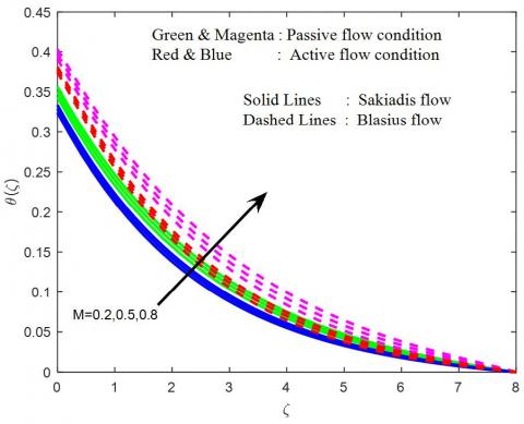
Figure 4. Temperature profiles for different values of $B i_{1}$
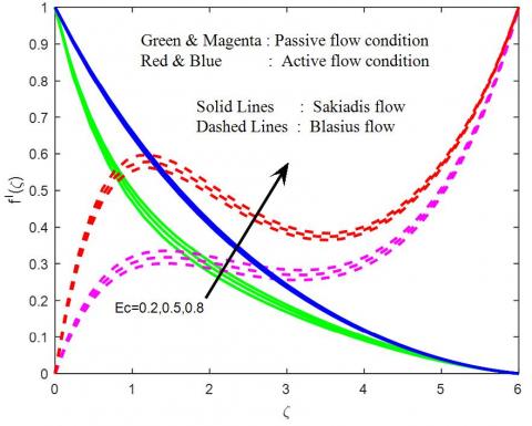
Figure 5. Velocity profiles for different values of Ec
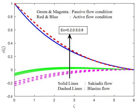
Figure 6. Temperature profiles for different values of Ec
The influence of thermophoresis parameter on velocity, temperature and concentration profiles are shown in Figures 2-4. It will watch that velocity and temperature distributions to improve for Blasius and Sakiadis flow in the presence of passive and active flow condition and decline the concentration distributions in both cases. It is interesting to observe that active flow condition shows higher momentum boundary layer compared to passive flow condition for both the cases of Blasius and Sakiadis respectively. Figures 5-7 illustrate the velocity, temperature and concentration distributions for different values of Eckert number. For small values of Eckert number enhances the momentum, thermal and concentration boundary layer thickness. The temperature in the flow region accelerates with increase in Eckert number. It is due to fact that heat energy is stored in the liquid due to frictional heating. The same phenomena can find in velocity and concentration distributions. We also observed that the active flow is higher than passive flow for velocity and temperature in Blasius and Sakiadis fluid flow cases.
Figure 7. Concentration profiles for different values of Ec
Figure 8. Velocity profiles for different values of Kr
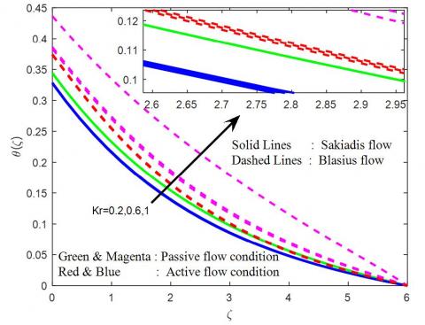
Figure 9. Temperature profiles for different values of Kr
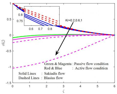
Figure 10. Concentration profiles for different values of Kr
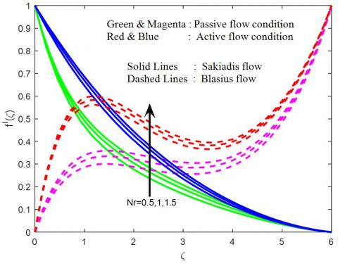
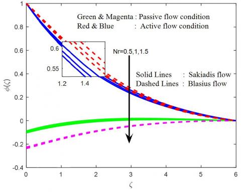
Figure 11. Velocity profiles for different values of Nr
Figure 12. Temperature profiles for different values of Nr
The chemical reaction effect on velocity, temperature and concentration profiles are presented in Figures 8-10. It is obviously notice that the higher values of chemical reaction parameter rise in velocity and temperature profiles while decrease in concentration profiles. In general, the higher values of chemical reaction to fall the molecular diffusivity. They are obtained by species transfer; an increase in chemical reaction parameter decelerates species concentration distribution. The concentration profiles decrease at all points of the fluid flow field with rise in chemical reaction parameter for both Blasius and Sakiadis fluid flows (see in Figure 10).
Figure 13. Concentration profiles for different values of Nr
Figure 14. Velocity profiles for different values of M
Figure 15. Temperature profiles for different values of M
Figures 11-13 demonstrate the influence of thermal radiation parameter on velocity, temperature and concentration distributions within the boundary layer. It is noticed that the fluid temperature increases as thermal radiation increases due to the fact that the temperature increases conduction effect of the nanofluid in the presence of thermal radiation. Therefore, higher values of radiation parameter imply higher surface heat flux and so, increase the temperature within the thermal boundary region. It is also observed that the thermal boundary layer thickness increases with increasing the values of thermal radiation parameter, as well as same phenomena can be observed in velocity field. The opposite trend can be observed in concentration field (Figure 13). The active flow is higher than the passive flow in concentration profiles has been observed in both Blasius and Sakiadis flow cases.
Figure 16. Concentration profiles for different values of M
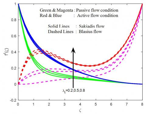
Figure 17. Velocity profiles for different values of $\lambda_{T}$
It is observed that the various values of the magnetic field parameter, we can notice that increase in M decelerates the velocity and enhances in temperature and concentration fields are seen in Figures 14-16. Physically, this result quantitatively agrees with expectations. This is due to fact that the application of magnetic field on an electrically conducting fluid give rise to resistive type force (retardation force) is known as Lorentz force. This force has tendency to slow down the motion of the boundary layer and to enhance increase in concentration and temperature distributions in both Blasius and Sakiadis fluid flows.
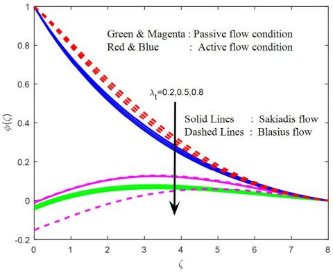
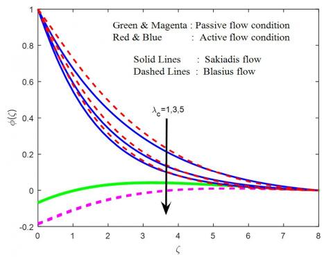
The influence of thermal and solutal buoyancy parameters on velocity, temperature and concentration fields are shown in Figures 17-22. It is noticed that an increase in thermal and solutal buoyancy parameters are leads to a rise in the fluid velocity due to enhancement in buoyancy force (see in Figures 17 and 20) and decelerates in remaining temperature and concentration distributions are shown in Figures 18-19 and 21-22. Here, the positive values of thermal and solutal buoyancy parameter correspond to cooling of the plate. In addition, it is observed that the velocity increases sharply near the wall as thermal and solutal buoyancy increases. It is expected that the fluid velocity increases and the peak value becomes more distinctive due to increase in the buoyancy force represented by thermal and solutal buoyancy parameter for both Blasius and Sakiadis fluid flow cases.
Figure 18. Temperature profiles for different values of $\lambda_{T}$
Figure 19. Concentration profiles for different values of $\lambda_{T}$
From Table 1 we have to see that the present results are good agreement with compared previous results in the absence of Eckert number, porosity parameter, chemical reaction parameter, thermal radiation parameter and Biot numbers with Grubka and Bobba [16], Ali [17], and Ishak [18] in both Blasius and Sakiadis flow cases. In present results discussed the effects of physical parameters namely thermal buoyancy parameter and Prandtl number on heat transfer characteristics.
The nature of Sakiadis and Blasius flow active passive control modulating quantities on friction factor coefficient, Nusselt and Sherwood numbers are reencountered through is shown in Table 2. It is evident that for friction factor coefficient and heat transfer rates increases with increase in Biot number, thermal radiation parameter and thermal buoyancy parameter intensifies but chemical reaction parameter, magnetic field parameter exhibits an opposite outcome; finally for mass transfer rate a gain in the magnitude of Eckert number, chemical reaction parameter, solutal buoyancy parameter for both the cases of active passive control of Sakiadis and Blasius flow conditions.
Figure 20. Velocity profiles for different values of $\lambda_{c}$
Figure 21. Temperature profiles for different values of $\lambda_{c}$
Figure 22. Concentration profiles for different values of $\lambda_{c}$
Table 1. Comparison of some of the values of wall temperature gradient $-\theta^{\prime}(0)$ with the present results in the absence of thermal radiation when $E c=K=B i_{1}=K r=N r=0$
|
$\lambda_{T}$ |
Pr |
Grubka and Bobba [16] |
Ali [17] |
Ishak et al. [18] |
Present results |
|
|
0.01 |
0.0197 |
|
0.0197 |
0.019723 |
|
|
0.72 |
0.8086 |
0.8058 |
0.8086 |
0.808836 |
|
0.0 |
1.0 |
1.0000 |
0.9961 |
1.00000 |
1.000000 |
|
|
3.0 |
1.9237 |
1.9144 |
1.9237 |
1.923687 |
|
|
10.0 |
3.7207 |
3.7006 |
3.7207 |
3.720788 |
|
|
10.0 |
12.2940 |
|
12.2941 |
12.30039 |
|
0.0 |
1.0 |
|
|
1.6820 |
1.681921 |
|
1.0 |
|
|
|
1.7039 |
1.703910 |
|
1.0 |
1.0 |
|
|
1.0873 |
1.087206 |
|
2.0 |
|
|
|
1.1423 |
1.142298 |
|
3.0 |
|
|
|
1.1853 |
1.185197 |
Table 2. Numerical values of skin friction coefficient, Nusselt and Sherwood numbers for various values of parameters
|
Blasius flow |
||||||||||||
|
$B i_{1}$ |
Ec |
Kr |
Nr |
M |
$\lambda_{t}$ |
$\lambda_{c}$ |
$\mathrm{Re}_{x}^{1 / 2} \mathrm{Cf}$ |
$\mathrm{Re}_{x}^{-1 / 2} \mathrm{Nu}$ |
$\mathrm{R} \mathrm{e}_{x}^{-1 / 2} \mathrm{Sh}$ |
|||
|
Passive flow |
Active flow |
Passive flow |
Active flow |
Passive flow |
Active flow |
|||||||
|
0.2 |
|
|
|
|
|
|
-0.929088 |
-0.407278 |
0.983749 |
1.017944 |
-0.087444 |
0.405543 |
|
0.3 |
|
|
|
|
|
|
-0.809852 |
-0.284497 |
1.282986 |
1.326306 |
-0.114043 |
0.409942 |
|
0.4 |
|
|
|
|
|
|
-0.720460 |
-0.194725 |
1.515378 |
1.564209 |
-0.134700 |
0.412418 |
|
|
0.2 |
|
|
|
|
|
-0.929088 |
-0.407278 |
0.983749 |
1.017944 |
-0.087444 |
0.405543 |
|
|
0.5 |
|
|
|
|
|
-0.888899 |
-0.393068 |
0.958808 |
1.006237 |
-0.085227 |
0.406598 |
|
|
0.8 |
|
|
|
|
|
-0.853745 |
-0.379517 |
0.936746 |
0.995112 |
-0.083266 |
0.407598 |
|
|
|
0.2 |
|
|
|
|
-0.929088 |
-0.407278 |
0.983749 |
1.017944 |
-0.087444 |
0.405543 |
|
|
|
0.6 |
|
|
|
|
-0.927670 |
-0.412626 |
0.983776 |
1.016789 |
-0.087447 |
0.433790 |
|
|
|
1.0 |
|
|
|
|
-0.926394 |
-0.417605 |
0.983804 |
1.015717 |
-0.087449 |
0.460601 |
|
|
|
|
0.5 |
|
|
|
-0.929088 |
-0.407278 |
0.983749 |
1.017944 |
-0.087444 |
0.405543 |
|
|
|
|
1.0 |
|
|
|
-0.882309 |
-0.359484 |
1.260719 |
1.299859 |
-0.084048 |
0.423177 |
|
|
|
|
1.5 |
|
|
|
-0.845865 |
-0.323240 |
1.527465 |
1.570467 |
-0.081465 |
0.436280 |
|
|
|
|
|
0.2 |
|
|
-0.727182 |
-0.280966 |
0.993495 |
1.024713 |
-0.087509 |
0.424378 |
|
|
|
|
|
0.5 |
|
|
-0.839288 |
-0.407278 |
0.983534 |
1.017944 |
-0.086616 |
0.405543 |
|
|
|
|
|
0.8 |
|
|
-0.943148 |
-0.525086 |
0.974132 |
1.011284 |
-0.085774 |
0.387858 |
|
|
|
|
|
|
0.2 |
|
-1.297331 |
-0.795885 |
0.918791 |
0.986735 |
-0.080821 |
0.315997 |
|
|
|
|
|
|
0.5 |
|
-1.244352 |
-0.750115 |
0.928291 |
0.990488 |
-0.081671 |
0.326395 |
|
|
|
|
|
|
0.8 |
|
-1.191713 |
-0.705167 |
0.937165 |
0.994033 |
-0.082465 |
0.336238 |
|
|
|
|
|
|
|
1.0 |
-0.839288 |
-0.395794 |
0.983534 |
1.015007 |
-0.086616 |
0.395601 |
|
|
|
|
|
|
|
3.0 |
-0.874469 |
0.382782 |
0.985914 |
1.045174 |
-0.086829 |
0.496358 |
|
|
|
|
|
|
|
5.0 |
-0.914188 |
1.105639 |
0.987300 |
1.054173 |
-0.086953 |
0.559191 |
The present analysis investigates a problem with influences of different parameters on fluid velocity, temperature and concentration for both Sakiadis and Blasius fluid flow cases. The presented analysis also elaborates the features of variable thermal conductivity and viscous dissipation, chemical reaction is taken into account. Based on the present investigation the following observations are made:
[1] Ibrahim, W. (2016). Passive control of nanoparticle of micropolar fluid past a stretching sheet with nanoparticles, convective boundary condition and second-order slip. Journal of Process Mechanical Engineering, 231(4): 1-16. https://doi.org/10.1177/0954408916629907
[2] Tripathi, R., Seth, G.S., Mishra, M.K. (2017). Double diffusive flow of a hydromagnetic nanofluid in a rotating channel with Hall effect and viscous dissipation: Active and passive control of nanoparticles. Advanced Powder Technology, 28(10): 2630-2641. https://doi.org/10.1016/j.apt.2017.07.015
[3] Acharya, N., K. Das, K., Kund, P.K. (2017). Fabrication of active and passive controls of nanoparticles of unsteady nanofluid flow from a spinning body using HPM. The European Physical Journal Plus, 132: 323. https://doi.org/10.1140/epjp/i2017-11629-y
[4] Hayat, T., Aziz, A., Muhammad, T., Alsaedi, A. (2017). Active and passive controls of Jeffrey nanofluid flow over a nonlinear stretching surface. Results in Physics, 7: 4071-4078. https://doi.org/10.1016/j.rinp.2017.10.028
[5] Halim, N.A., Haq, R.U., Noor, N.F.M. (2017). Active and passive controls of nanoparticles in Maxwell stagnation point flow over a slipped stretched surface. Meccanica, 52(7): 1527-1539. https://doi.org/10.1007/s11012-016-0517-9
[6] Halim, N.A., S. Sivasankaran, S., Noor, N.F.M. (2016). Active and passive controls of the Williamson stagnation nanofluid flow over a stretching/shrinking surface. Neural Computing & Applications, 28(Supplement 1): 1023-1033. https://doi.org/10.1007/s00521-016-2380-y
[7] Wagner, T., Kroll, A., Haramagatti, C.R., Lipinski, H.G., Wiemann, M. (2017). Classification and segmentation of nanoparticle diffusion trajectories in cellular micro environments. Plos One, 12(1): e0170165. https://doi.org/10.1371/journal.pone.0170165
[8] Muhammad, T., Alsaedi, A., Shehzad, S.A., Hayat, T. (2017). A revised model for Darcy-Forchheimer flow of Maxwell nanofluid subject to convective boundary condition. Chinese Journal of Physics, 55(3): 963-976. https://doi.org/10.1016/j.cjph.2017.03.006
[9] Kuo, B.L. (2004). Thermal boundary-layer problems in a semi-infinite flat plate by the differential transformation method. Applied Mathematics and Computation, 150(2): 303-320. https://doi.org/10.1016/S0096-3003(03)00233-9
[10] Hossain, M.A., Khanafer, K., Vafai, K. (2001). The effect of radiation on free convection flow of fluid with variable viscosity from a porous vertical plate. International Journal of Thermal Science, 40(2): 115-124. https://doi.org/10.1016/S1290-0729(00)01200-X
[11] Raptis, A., Perdikis, C., Takhar, H.S. (2004). Effect of thermal radiation on MHD flow. Applied Mathematics and Computation, 153(3): 645-649. https://doi.org/10.1016/S0096-3003(03)00657-X
[12] Bataller, R.C. (2008) Radiation effects for the Blasius and Sakiadis flows with a convective surface boundary condition. Applied Mathematics and Computation, 206(2): 832-840. https://doi.org/10.1016/j.amc.2008.10.001
[13] Fang, T., Yao, S., Pop, I. (2011). Flow and heat transfer over a generalized stretching/shrinking wall problem-Exact solution of the Navier-Stokes equations. International Journal of Non-Linear Mechanics, 46(9): 1116-1127. https://doi.org/10.1016/j.ijnonlinmec.2011.04.014
[14] Garg, P., Purohit, G.N., Choudary, R.C. (2015). A similarity solution for laminar thermal boundary layer over a flat plate with internal heat generation and a convective surface boundary condition. Journal of Rajasthan Academy of Physical Sciences, 14(4): 221-226. https://doi.org/10.1016/j.cnsns.2008.05.003
[15] Vajravelua, K., Prasadb, K.V., Ng, C.O. (2013). Unsteady convective boundary layer flow of a viscous fluid at a vertical surface with variable fluid properties. Nonlinear Analysis: Real World Applications, 14(1): 455-464. https://doi.org/10.1016/j.nonrwa.2012.07.008
[16] Grubka, L.J., Bobba, K.M. (1985). Heat transfer characteristics of a continuous, stretching surface with variable temperature. J. Heat Transfer, 107(1): 248-250. https://doi.org/10.1115/1.3247387
[17] Ali, M.E. (1994). Heat transfer characteristics of a continuous stretching surface. Warme and Stoffubertragung, 29(4): 227-234. https://doi.org/10.1007/BF01539754
[18] Ishak, A., Nazar, R., Pop, I. (2009) Boundary layer flow and heat transfer over an unsteady stretching vertical surface. Meccanica, 44(4): 369-375. https://doi.org/10.1007/s11012-008-9176-9
[19] Brewster, M.Q. (1972). Thermal Radiative Transfer Properties. John Wiley and Sons.
[20] Mabood, F., Shafiq, A., Hayat, T., Abelman, S. (2017). Radiation effects on stagnation point flow with melting heat transfer and second order slip. Results in Physics, 7: 31-42. https://doi.org/10.1016/j.rinp.2016.11.051
[21] Chiam, T.C. (1996). Heat transfer with variable thermal conductivity in a stagnation point flow towards a stretching sheet. International Communications in Heat Mass Transfer, 23(2): 239-248. https://doi.org/10.1016/0735-1933(96)00009-7
[22] Raptis, A., C. Perdikis, C. (1991). Viscoelastic flow by the presence of radiation. Journal of Applied Mathematics and Mechanics, 78: 277-279. https://doi.org/10.1002/(SICI)1521-4001(199804)78:4<277::AID-ZAMM277>3.0.CO;2-F
[23] Mabood, F., Shateyi, S., Rashidi, M.M., Momoniat, E., Freidoonimehr, N. (2016). MHD stagnation point flow heat and mass transfer of nanofluids in porous medium with radiation, viscous dissipation and chemical reaction. Advanced Powder Technology, 27(2): 742-749. https://doi.org/10.1016/j.apt.2016.02.033
[24] Perdikis, C., Raptis, A. (1996). Heat transfer of a micro polar fluid by the presence of radiation. Heat Mass Transfer, 31(6): 381-382. https://doi.org/10.1007/BF02172582
[25] Makinde, O.D., Mabood, F., Ibrahim, S.M. (2018). Chemically reacting on MHD boundary layer flow of nanofluids over a nonlinear stretching sheet with heat source/sink and thermal radiation. THERMAL SCIENCE, 22(1): 495-506. https://doi.org/10.2298/TSCI151003284M
[26] Raptis, A. (1999). Radiation and viscoelastic flow. International Communications in Heat Mass Transfer, 26(6): 889-895. https://doi.org/10.1016/S0735-1933(99)00077-9