Marco Ferraro | Girolama Airò Farulla* | Giovanni Tumminia | Francesco Guarino | Davide Aloisio | Giovanni Brunaccini | Francesco Sergi | Fabio Giusa | Antonio Emanuel Colino | Maurizio Cellura | Vincenzo Antonucci
OPEN ACCESS
Ventilated Façades integrating photovoltaic panels are a promising way to improve efficiency and the thermal-physical performances of buildings. Due the inherent intermittence of the non-programmable renewable energy sources, their increasing usage implies the use of energy storage systems to mitigate the mismatch between power generation and the buildings’ load demand. The main purpose of this paper is to investigate the thermo-fluid dynamic performances of a prototype integrating a photovoltaic cell and a battery as a module of an active ventilated façade. Based on an experimental setup, a numerical study in steady state conditions of flow through the air cavity of the module has been carried out and implemented in a fluid-dynamics Finite Volume code. In order to assess the viability of the prototype, the calibrated model was lastly used to predict thermal performance of the prototype on different climate conditions supporting its further improvement.
BIPV, battery, ventilated façade, CFD
Achieving high energy efficiency within the building sector is the ambitious focus of several policy and research actions at international level [1, 2]. The construction of nearly-zero energy buildings (nZEB) [3, 4] and retrofitting solutions in the existing building stock are playing a key role both to achieve a higher level of self-sufficiency and to improve the energy performance of buildings [5-7]. External thermal insulation composite system and ventilated façades are among some of the practical solutions available for the retrofit of existing buildings [8]. Several studies showed that ventilated façades integrated with Photovoltaic (PV) systems are among the promising ways of the Building Integrated Photovoltaic (BIPV) system to improve both the thermal-physical performances of t existing buildings and PV conversion efficiency [9, 10]. The major benefit of this integration is that PV panels shading the building reduce heat gain from solar radiation while the air cavity, facilitating the buoyancy force resulted from the solar radiation, induces the ambient air into the channel with positive effect on the PV temperature [11].
However, the major limit of non-programmable renewable energy sources is the discontinuity in the production of electricity. Energy storage is paramount to allow renewable energies to be more competitive within the current market [12, 13]. The increasing use of renewable energy systems might be easier and more effective under the adoption of energy storage systems to mitigate the mismatch between the power generation and the building’s demand [14, 15]. Batteries are the most used technology to store energy and their integration with a PV panel as a whole system is a flexible and already viable solution [16]. The whole system PV- batteries lead to each PV module can be treated as a self-rechargeable unit. However, in order to avoid the degradation of the efficiency of the entire system each battery must be at the proper working temperature to avoid damages and accelerated degradation [17].
Many aspects of ventilated façades have been studied theoretically and experimentally such as the effects of the air gap behind PV wall on the buoyancy and induced ventilation rate [18], effects of the PV panel orientation and wind direction on the overall performance of the BIPV [19]. In literature, Computational Fluid Dynamic (CFD) was utilized as the main method to achieve accurate and detailed results in thermal performance estimation for ventilated PV façades.
Sandberg and Moshfegh [20] performed CFD simulations of vertical façades to derive temperature and velocity profiles in air gaps behind photovoltaic panels. Moreover, empirical correlations for the mass flow rate, air velocity and temperature increase were obtained through the analysis of experimental data.
Peng et al. [21] performed CFD simulations to evaluate the overall performance of a semi-transparent ventilated PV façade under different air velocity conditions. They showed that buoyancy-driven ventilated mode performed better than natural convection for improving the PV performances and reducing the solar heat gain.
Goverde et al. [22, 23] investigated the effects of wind on PV modules in terms of power output of the photovoltaic system. Their results showed that a decreasing in wind velocity leads to a lower heat transfer coefficient. As consequence, an increase of PV cells temperature results in a reduction both in the photovoltaic conversion efficiency and the maximum output power.
In this context, the paper presents the thermo-fluid dynamics performance of a prototype of an active ventilated façade integrating PV module and a lithium battery starting from a previous preliminary authors’ work [24]. CFD steady state simulations have been performed to investigate the effects of the buoyancy-induced by the thermal gradients within the air cavity of ventilated façade. The numerical model developed to investigate the airflow and temperature distributions was implemented in the multi-physics Finite Volume Code Ansys Fluent. The model has been calibrated and validated on experimental data.
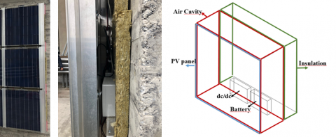
Figure 1 shows some pictures of the prototype installed and its constructive scheme, while Table 1 reports the geometrical dimensions of a single module consisting of a PV module as external façade, a Li-ion battery and a dc-dc converter contained in two casings fixed on the insulation layer.
Figure 1. Schematic of the prototype
Table 1. Geometrical dimensions of the prototype
|
Parameters |
Values |
|
PV panel dimensions (mm) |
680 x 680 x 7 |
|
PV thickness (mm) |
7 |
|
Glass thickness (mm) |
3.2 |
|
Eva thickness (mm) |
0.2 |
|
PV cells thickness (mm) |
0.2 |
|
Air cavity thickness (cm) |
25 |
|
Insulation thickness (cm) |
10 |
|
Casing volume (cm3) |
18 x 13 x 4 |
The PV panel used has the stratification layers shown in Figure 2. In Table 2 are listed the electrical features of the PV module simulated.
Figure 2. Schematic of the PV panel layers
The two casings, fixed on the insulation, contain a battery and an integrated control board comprising a MPPT (Maximum Power Point Tracker), a bidirectional battery charger (DC/DC) and a diode (Shottky).
Table 2. Electrical features of PV
|
Parameters |
Values |
|
Cell’s number |
16 arranged in series |
|
Nominal Voltage (V) |
8.5 |
|
Nominal Current (A) |
7.5 |
|
Voltage Coefficient (mV/°C) |
122 |
|
Current Coefficient |
4.36 |
|
Efficiency |
14% |
Both battery and control board act as heat source dissipating the generated heat through the casings. To ensure the electrical and electronic components operate within the nominal surrounding temperatures a proper cooling effect must be guaranteed. Installing the casings within an air cavity has the main advantage that heat dissipation is facilitated by natural convection leading to lower operation temperatures [25].
The physical properties [26] of each material utilized in the proposed prototype are listed in Table 3.
Table 3. Properties of prototype’s components materials
|
|
|
Property |
||
|
Material |
Component |
ρ(kg/m3) |
Cp(J/(kg K) |
λ(W/(m K)) |
|
Glass |
PV module |
2500 |
750 |
1.04 |
|
Polycrystallin Silicium |
PV module |
2330 |
700 |
150 |
|
EVA |
PV module |
2500 |
0.29 |
0.35 |
|
Polypropylene |
Casings |
1030 |
1040 |
0.16 |
|
Rockwood |
Insulation layer |
100 |
1030 |
0.035 |
Both geometrical dimensions and physical properties were used to develop a numerical heat transfer 3D model with temperature dependent air properties.
The following modeling hypothesis has been made:
In Figure 3 a schematic representation of the boundary conditions assumed is shown:
Figure 3. Schematic of boundary conditions
For solar radiation on vertical surface, air velocity and wind velocity, used as inputs of the simulations, both experimental and meteorological data were used.
The volumetric heat dissipation (W/m3) in the PV panel was estimated as followed [26]:
$q_{P V}=\alpha_{g l a s s} G_{P V} A\left(1-\eta_{P V}\right)$ (1)
where aglass is the absorptivity of the glass, GPV the vertical solar radiation on the PV panel (W/m2), A the area of the PV panel (m2), hPV the efficiency of the PV panel. In accordance to [27] aglass was assumed 0.9 in this work.
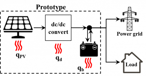
Figure 4 illustrates the electrical connection between the different components, indicating the power flows and the heat generated by each component with an overview of relevant nomenclature. The volumetric heat dissipation of DC-DC (qd) and battery (qb) were estimated using equations (2) and (3), respectively:
$q_{d}=\left(1-\eta_{d}\right) P_{P V}+i^{2} r$ (2)
$q_{b}=\left(1-\eta_{b}\right) \eta_{a} P_{P V}$ (3)
where PPV is the power generated by the PV panel (W), i the current (A) generated by the panel, r the electrical resistance of the diode, ηd and ηb the efficiency of the DC/DC and battery respectively.
To determine the heat generated into the battery during the charge and discharge phases, ηb has been defined as a function of the current through the battery and modeled by the equation (4):
$\eta_{b}=f(i)$ (4)
A set of tests was performed to identify the correlation between ηb and the current flowing into the battery. ηd has been assumed equal to 0.95 according to [30] and r to 0.08 mΩ according to [31].
Figure 4. Schematic of electrical connection among PV panel, diode and battery
2.1 Mathematical model
The mathematical model for the prototype proposed in this paper can be divided into:
2.1.1 Fluid model
The partial differential Navier-Stokes equations describe the flow of an incompressible fluid. Based on 3D space rectangular coordinate system, for a Newtonian fluid in steady state conditions these are given as in the following [32]:
$\frac{\partial u_{i} u_{j}}{\partial x_{j}}=\frac{1}{\rho} \frac{\partial p}{\partial x_{i}}+\frac{\partial}{\partial x_{j}} v\left(\frac{\partial u_{i}}{\partial x_{j}}+\frac{\partial u_{j}}{\partial x_{i}}\right)-\frac{2}{3} \frac{\partial}{\partial x_{j}} v \nabla \mathbf{u}+g_{i}$ (5)
where ρ is the fluid density (kg/m3), p is the pressure (Pa), u the velocity vector (m/s), ν the coefficient of kinematic viscosity (N s/m2), g the gravity acceleration (m/s2).
2.1.2 Heat transfer model
Solar radiation on the PV module is partly reflected by the external tempered glass layers and partly absorbed by the solar cell layers. The solar energy not absorbed by the solar cells to be partly converted into direct current (DC) electricity is dissipated as waste heat towards both the external environmental and inside the air cavity.
Within the solid parts of the system, i.e. PV module, casings and wall insulation the conduction heat transfer (Fourier’s low), in steady state conditions, is given as in the following [33, 34]:
$\frac{\partial}{\partial x_{j}} \lambda_i \frac{\partial T}{\partial x_{j}}+q_{i}=0$ (6)
where λi is the thermal conductivity of each part (W/(m K) and qi the volumetric heat generation (W/ m3).
For the PV panel, dc-dc and battery q is given by Eqns. (1), (2) and (3), respectively.
In the air cavity, the heat exchange with the backside tempered glass layer of the PV panel (backsheet) and the front side of the insulation is dominated by the conductive and convective heat transfer. The convective heat transfer equation is given as followed:
$q_{c}=h_{i}\left(T_{s}-T_{a}\right)$ (7)
where hi is the convective heat transfer coefficient (W/(m2K)), Ti temperature of each surface wall in contact with the air moving into the channel (°C), Ta the temperature of the air inside the cavity (°C).
On the external surface of the PV panel the free convective heat transfer coefficient is given by [27]:
$h_{f i e e}=\frac{\lambda_{g l a s s}}{L}\left\{0.825+\frac{0.387 R a^{1/6}}{\left[1+(0.492 / \mathrm{Pr})^{9 / 16}\right]^{8 / 27}}\right\}^{2}$ (8)
where λglass is the thermal conductivity of the temperate glass cover (W/(m K)), L is the height of PV panel (m), Ra the Raleigh number, Pr the Prandtl number.
$R a=\frac{g \beta \Delta T L^{3}}{\alpha v}$ (9)
$\operatorname{Pr}=\frac{v}{\alpha}$ (10)
where a is the thermal diffusivity (N s/m2), b is the thermal expansion coefficient (1/K), DT the temperature difference between the external surface of the PV panel and air temperature.
The numerical model was implemented in the multi-physics Finite Volume Code Ansys Fluent. To avoid the mesh dependency program, a grid sensitive analysis was conducted and a mesh of about 500K elements was used for the simulations. In the Fluent solver, RNG k-e model was selected in the Viscous Model and Enhanced Thermal Treatment was active in near-wall treatment. Coupled algorithm was used in pressure-velocity coupling. Second Order Upwind was selected in momentum and energy equations. A convergence criterion of 10-5 was applied to the residuals of continuity equations while for the momentum and energy ones was 10-6 [23]. The model was developed to evaluate, on each surface, both the weighted average temperature T value and the temperature distribution T (xi, Ti), reported in Eq. 11
$T=\frac{\sum_{i} A_{i} T_{i}}{\sum_{i} A_{i}}$ (11)
where i is the generic mesh element, A and Ti the area of the i-element and the temperature evaluated in its centroid, xi the position vector.
Average temperature values were calculated and validated by the experimental data while the temperature distribution.
2.2 Experimental tests
The PV mathematical model, aiming to predict the temperature on its surfaces, has been validated in a previous author’s work [21]. In this study, tests have been carried out to identify and validate a simplified battery model and to validate the temperature profile of the whole prototype.
2.2.1 Test results on battery
The Lithium Titanate parallelepiped shape battery is composed by nano-scale LTO (Li4Ti5O12) in the anode and NCM (LiNi0.5Co0.2Mn0.3O2) with the following features: 2.7 V 23 Ah.
The battery has been tested with a Potentiostat Autolab PGSTAT302N equipped with a Booster system to raise the current set points up to ±20A. The software suite Nova 2.1 has been used to realize test procedures and record data coming from the cell.
The battery temperature has been controlled via a climatic chamber (Angelantoni mod. 600 L) and monitored by a Pt100 thermistor.
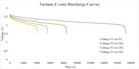
The charge/discharge rates affect the electrochemical process into a battery causing a reduction in efficiency. Charging/discharging tests at different current values were carried out to assess battery performance with different charge/discharge currents at 25 °C Figure 5.
(a)
(b)
Figure 5. Charge (a) and discharge (b) curves at 25 °C for LTO cell
Discharge test were performed starting from 100 % SoC with constant current set-point (galvanostatic-mode) until reaching the lower cutoff voltage. The 100 % SoC is reached by performing charge cycles with a galvanostatic phase until the upper voltage threshold is reached, followed by a potentiostatic phase at upper cutoff voltage until the current goes under 0.01 A. This phase is needed due to typical voltage hysteresis of batteries, which increase/decrease operative voltage during charge/discharge phases, to fully charge the same.
The energy efficiency has been calculated with the following equation at various c-rate:
$\eta_{b}=\frac{E_{\text {discharged}}}{E_{\text {charged}}}$ (12)
where
$E=\int_{t} v(t) i(t) d t$ (13)
The formula takes into account the energy loss in charge/discharge processes. In this work, it has been fully attributed to heat generation. The following Table 4 reports the efficiency at different charge/discharge currents.
Table 4. Battery efficiency at different charge/discharge rates at 25 °C
|
Charge/discharge current rates (Ampere) |
5 |
10 |
15 |
20 |
|
Efficiency |
0.9657 |
0.9281 |
0.8991 |
0.8740 |
The polynomial formula interpolating the experimental data is reported as the following equation (12), used to calculate the heat generated by the battery during its operation:
$\left\{\begin{array}{l}{\eta_{b}=0.97(i<5 A)} \\ {\eta_{b}=0.0001 i^{2} 0.0092 i+1.0084(i<5 A)}\end{array}\right.$ (14)
2.2.2 Test results on the whole prototype
To calibrate and validate the thermal model of the prototype, by comparing the monitored data to that of the model on the same time using recorded weather data as a model input, monitoring studies have been developed on the prototype. Monitoring was performed during 2019 for five days, from April 17th to April 21th.
Figure 6. Sensors position during the prototype monitoring. T1= external temperature of the PV panel, T2= temperature of the backsheet of the PV panel, T3= temperature of the inner insulation in contact with the air moving into the channel, T4= temperature of the external insulation
Figure 6 shows the monitored prototype, the installed sensors and their nomenclature. In detail, four thermocouples (chromel–alumel thermocouples (type k)), installed on both sides of the PV module and on both sides of the insulation layer, were used.
As showed in Figure 6, a weather station was installed near the prototype, recording global horizontal radiation, dry bulb temperature, wind velocity and direction. The solar radiation on a vertical south oriented surface was calculated from the measured global horizontal radiation on horizontal surfaces using the mathematical model developed by Perez et al. [36].
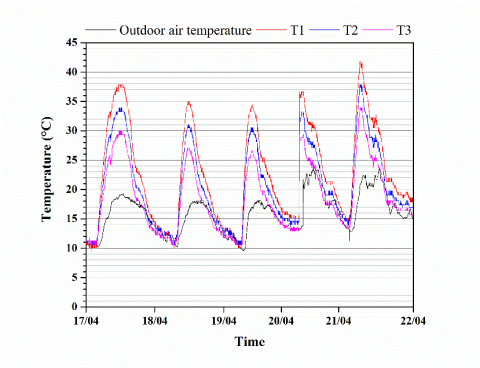
In Figure 7 the monitored weather data are shown. The outdoor air temperature varies between 9.6 °C and 23.6 °C, while T1 (the frontsheet temperature of the PV module) varies between 9.4 °C and 41.8 °C.
Figure 7. Monitored weather data for 5 days (April 17-21, 2019)
2.3 Model validation
The validation of the model was performed by comparing monitored and simulated data for one day of the monitored period (April 19, 2019) obtaining limited differences. Figure 8 shows the outdoor air temperature, the global horizontal radiation and the solar radiation on a vertical south oriented surface for the selected day.
Figure 8. Outdoor monitored weather data for the April 19th 2019
In all cases the differences are below 1.36 °C. In 90 % of the data, the absolute error is below 1.08 °C while for 50 % of the calibration data it is below 0.48 °C.
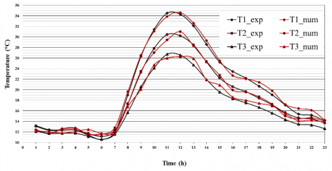
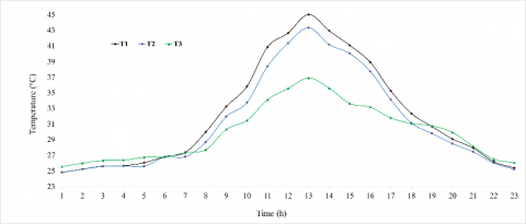
The following graph (Figure 9) reports the monitored temperatures (black lines) and the simulated average surface temperatures (red lines) for the 19th April 2019. During this day, there is a good agreement between simulated data and monitored data (the difference between the monitored and the simulated temperature is between -1.04 °C (T1) and +1.36 °C (T3).
To validate the results produced from the thermal model statistical techniques were employed as a method to assess the accuracy of outputs. Table 5 includes the statistical metrics and their equations used to assess the modeling error: mean bias error (MBE), root mean square error (RMSE) and the coefficient of variation of the root mean square error (CV(RMSE)). In particular the MBE of the simulated temperature vary from -0.05 °C (T2) to 0.56 °C (T3) while the RMSE is equal to vary from 0.47 °C (T2) to 0.81 °C (T3).
Figure 9. Experimental and numerical data of the thermal profiles of PV panel and insulation
Table 5. Errors quantification between monitored and simulated data
|
Statistical metrics |
Equation |
Number of equations |
Validation results |
||
|
T1 |
T2 |
T3 |
|||
|
MBE (°C) |
$\frac{1}{n} \sum_{1}^{n}\left(T_{s, i}-T_{m, i}\right)$ |
(14) |
0.25 |
-0.05 |
0.56 |
|
RMSE |
$\sqrt{\frac{1}{n} \sum_{1}^{n}\left(T_{s, i}-T_{m, i}\right)^{2}}$ |
(15) |
0.61 |
0.47 |
0.81 |
|
CV(RMSE) |
$\frac{\sqrt{\frac{1}{n} \sum_{1}^{n}\left(T_{s, i}-T_{m, i}\right)^{2}}}{\overline{T_{m}}}$ |
(16) |
0.03 |
0.03 |
0.05 |
|
Symbols |
|
|
|
|
|
|
Ts,i = Simulated temperature |
|||||
|
Tm,i = Monitored temperature |
|||||
|
$\overline{T_{m}}$ = Mean of the monitored temperatures |
|||||
The validated model allows studying the temperature gradient within the prototype‘s components and to check the temperatures in the worst weather conditions.
In the following Figure 10 the simulated insulation temperature distributions are shown.
|
a. 8:00 G=110 W/m2, Ta=14 °C |
b. 11:00 G=430 W/m2, Ta=18 °C |
|
c. 13:00 G=500 W/m2, Ta=18 °C |
d. 15:00 |
Figure 10. Hourly temperature profile of inner insulation (April 19, 2019)
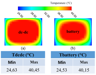
The presence of DC/DC and battery leads to a variation in the thermal profile of the inner insulation. For the simulated day (April 19, 2019) results show that the average surface temperature of the insulation is higher in contact with the casings containing the DC/DC and battery. The temperature surface of the casing containing the DC/DC is higher than that one containing the battery because the heat generated by the DC/DC (qd) is higher than the battery heat generation (qb). In Figure 11 the temperature distribution of the contact area of the two casings with the inner insulation is shown.
Figure 11. (a) Temperature distribution on the face of contact dc-dc- insulation and battery-insulation. (b) Minimum and maximum values of average temperature on these faces. Simulated case: G=500 W/m2, Ta=18 °C (h: 13:00)
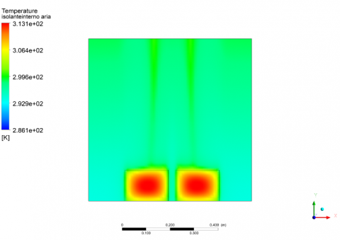
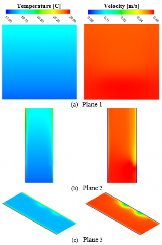
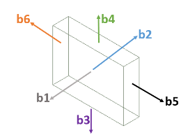
The air temperature distribution (Figure 13) within the air cavity was evaluated on the three mid-planes shown in Figure 12.
Figure 12. Planes to evaluate temperature and velocity distributions. Plane 1 of normal z, Plane 2 of normal x and Plane 3 of normal y
Figure 13. Air temperature and air velocity distributions (h: 13:00) on (a) plane 1 (b) plane 2 and (c) plane 3. The maximum temperature of about 30°C is reached both plane 2 and plane 3 in contact with the backsheet of the PV panel. The maximum velocity evaluated was 0.45 m/s
The model can be used to calculate the temperature profiles under the given operating condition, e.g. extreme weather conditions.
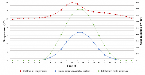
A simulation was carried out using climatic data, solar radiation and air temperature for a typical hot summer day. In particular, using a typical meteorological year for the weather station nearest the prototype, from the Building Technologies Office database of U.S. Department of Energy’s [37], the day (9th August) on which the maximum temperature occurs has been selected.
As shown in Figure 14, during this day the air temperature reaches the maximum value of 35 °C and never drops below 25 °C, even during the night hours.
Figure 14. Outdoor weather data used for the simulation.
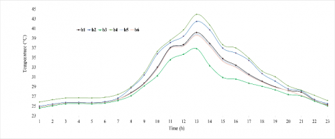
The following (Figure 15) shows the simulated temperature profiles during the entire day.
Figure 15. Thermal profiles of the prototype.
In particular, the six surfaces of the casing containing the battery have the thermal profiles reported in Figure 16. The temperature distributions obtained are comparable to thermal profiles evaluated by [17].
(a)
(b)
Figure 16. (a) Thermal profiles on the surface of the casing containing the battery during an entire day (August 9), (b) Schematic of the thermal zones of the casings
As shown in Figure 17, during the simulated day the average temperature reached by the surfaces of the battery casing are below those of the maximum battery operating temperature (⁓60 °C).
Figure 17. Temperature distribution on the face of contact battery-insulation. Simulated case: G=430 W/m2, Ta=34 °C (h: 13:00)Figure 17. Temperature distribution on the face of contact battery-insulation. Simulated case: G=430 W/m2, Ta=34 °C (h: 13:00)
This paper describes an innovative BIPV device integrating photovoltaic cells, a battery storing excess power and the needed electronics (MPPT and DC/DC converter). The distributed MPPT approach is suggested in literature among the main strategies to optimize the BIPV power generation.
In order to assess the thermal performance of the single integrated BIPV module a 3D model is developed and a test rig has been set-up to validate the model.
Besides the validation, the thermal performance of the panel has been evaluated during the hottest summer day obtained from a typical meteorological year for the same location.
The conclusions are summarized as follows:
The developed model and the test rig will be used to validate the prototype under different weather conditions and to assess the entire BIPV façade.
The study has been supported by the Ministry of Economic Development - Fund for sustainable growth (HORIZON 2020) - Project no. 181 “e-brick”.
|
A |
Area of the Photovoltaic panel |
|
CV(RMSE |
Coefficient of variation of the root mean square error |
|
G |
Vertical solar radiation (W/m2) |
|
g |
Gravity acceleration (m/s2) |
|
i |
Current (A) |
|
L |
Lenght of the Photovoltaic panel |
|
MBE |
Mean bias error |
|
p |
Pressure (Pa) |
|
Pr |
Prandtl number |
|
q |
Volumetric heat dissipation (W/m3) |
|
r |
Electrical resistance of the diode (W) |
|
Ra |
Raleigh number |
|
RMSE |
Root mean square error |
|
T |
Temperature (°C) |
|
u |
Vector velocity (m/s)
|
|
Greek symbols |
|
|
aglass |
Absorptivity of the glass |
|
a |
Thermal diffusivity (N s/m2) |
|
b |
Thermal expansion coefficient (1/K) |
|
ρ |
Fluid density (kg/m3) |
|
λ |
Thermal conductivity (W/(m K)) |
|
ν |
Coefficient of kinematic viscosity (N s/m2)
|
|
Subscripts |
|
|
a |
Air |
|
b |
Battery |
|
d |
Diode |
|
PV |
Photovoltaic |
|
s |
Surface |
[1] Papadopoulos, A.M. (2016). Forty years of regulations on the thermal performance of the building envelope in Europe: Achievements, perspectives and challenges. Energy Build, 127: 942-952. https://doi.org/10.1016/j.enbuild.2016.06.051
[2] Tronchin, L., Manfren, M., Nastasi, B. (2018). Energy efficiency, demand side management and energy storage technologies – A critical analysis of possible paths of integration in the built environment. Renew. Sustain. Energy Rev., 95: 341-353. https://doi.org/10.1016/J.RSER.2018.06.060
[3] Attia, S., Eleftheriou, P., Xeni, F., Morlot, R., Ménézo, C., Kostopoulos, V., Betsi, M., Kalaitzoglou, I., Pagliano, L., Cellura, M., Almeida, M., Ferreira, M., Baracu, T., Badescu, V., Crutescu, R., Hidalgo-Betanzos, J.M. (2017). Overview and future challenges of nearly zero energy buildings (nZEB) design in Southern Europe. Energy Build, 155: 439-458. https://doi.org/10.1016/j.enbuild.2017.09.043
[4] Cellura, M., Campanella, L., Ciulla, G., Guarino, F., Lo Brano, V., Cesarini, D.N., Orioli, A. (2011). The redesign of an Italian building to reach net zero energy performances: A case study of the SHC Task 40 - ECBCS Annex 52. In: ASHRAE Trans., pp. 331-339. https://doi.org/10.3390/buildings7030068
[5] Sozer, H. (2010). Improving energy efficiency through the design of the building envelope. Build. Environ, 45: 2581–2593. https://doi.org/10.1016/j.buildenv.2010.05.004
[6] Vigna, I., Pernetti, R., Pasut, W., Lollini, R. (2018). New domain for promoting energy efficiency: Energy Flexible Building Cluster, Sustain. Cities Soc., 38: 526-533. https://doi.org/10.1016/j.scs.2018.01.038
[7] Cellura, M., Ciulla, G., Guarino, F., Longo, S. (2017). Redesign of a rural building in a heritage site in Italy: Towards the Net Zero energy target. Buildings, 7(3): 68. https://doi.org/10.3390/buildings7030068
[8] Colinart, T., Bendouma, M., Glouannec, P. (2019). Building renovation with prefabricated ventilated façade element: A case study. Energy Build, 186: 221-229. https://doi.org/10.1016/J.ENBUILD.2019.01.033
[9] Lai, C.M., Hokoi, S. (2015). Solar Façades: A review. Build. Environ, 91: 152-165. https://doi.org/10.1016/J.BUILDENV.2015.01.007
[10] Zhang, T., Tan, Y., Yang, H., Zhang, X. (2016). The application of air layers in building envelopes: A review. Appl. Energy, 165: 707-734. https://doi.org/10.1016/J.APENERGY.2015.12.108
[11] Dubey, S., Sarvaiya, J.N., Seshadri, B. (2013). Temperature dependent photovoltaic (PV) efficiency and its effect on PV production in the world - A review. Energy Procedia, 33: 311-321. https://doi.org/10.1016/j.egypro.2013.05.072
[12] Thang, T.V., Ahmed, A., Kim, C.I., Park, J.H. (2015). Flexible system architecture of stand-alone PV power generation with energy storage device. IEEE Trans. Energy Convers, 30: 1386-1396. https://doi.org/10.1109/TEC.2015.2429145
[13] Li, P., Dargaville, R., Cao, Y., Li, D.Y., Xia, J. (2017). Storage aided system property enhancing and hybrid robust smoothing for large-scale PV systems. IEEE Trans. Smart Grid, 8: 2871-2879. https://doi.org/10.1109/TSG.2016.2611595
[14] Ould Amrouche, S., Rekioua, D., Rekioua, T., Bacha, S. (2016). Overview of energy storage in renewable energy systems. Int. J. Hydrogen Energy, 41: 20914-20927. https://doi.org/10.1016/J.IJHYDENE.2016.06.243
[15] Moshövel, J., Kairies, K.P., Magnor, D., Leuthold, M., Bost, M., Gährs, S., Szczechowicz, E., Cramer, M., Sauer, D.U. (2015). Analysis of the maximal possible grid relief from PV-peak-power impacts by using storage systems for increased self-consumption. Appl. Energy, 137: 567-575. https://doi.org/10.1016/J.APENERGY.2014.07.021
[16] Aneke, M., Wang, M. (2016). Energy storage technologies and real life applications – A state of the art review. Appl. Energy, 179: 350-377. https://doi.org/10.1016/j.apenergy.2016.06.097
[17] Hammami, M., Torretti, S., Grimaccia, F., Grandi, G. (2017). Thermal and performance analysis of a photovoltaic module with an integrated energy storage system. Appl. Sci., 7: 1107. https://doi.org/10.3390/app7111107
[18] Mingotti, N., Chenvidyakarn, T., Woods, A.W. (2011). The fluid mechanics of the natural ventilation of a narrow-cavity double-skin facade. Build Environ, 46: 807-823. https://doi.org/10.1016/j.buildenv.2010.09.015
[19] Kaplani, E., Kaplanis, S. (2014). Thermal modelling and experimental assessment of the dependence of PV module temperature on wind velocity and direction, module orientation and inclination. Sol. Energy, 107: 443-460. https://doi.org/10.1016/j.solener.2014.05.037
[20] Sandberg, M., Moshfegh, B. (2002). Buoyancy-induced air flow in photovoltaic facades: Effect of geometry of the air gap and location of solar cell modules. Build. Environ, 37: 211-218. https://doi.org/10.1016/S0360-1323(01)00025-7
[21] Peng, J., Lu, L., Yang, H., Ma, T. (2015). Comparative study of the thermal and power performances of a semi-transparent photovoltaic façade under different ventilation modes. Appl. Energy, 138: 572-583. https://doi.org/10.1016/J.APENERGY.2014.10.003
[22] Goverde, H., Goossens, D., Govaerts, J., Dubey, V., Catthoor, F., Baert, K., Poortmans, J., Driesen, J. (2015). Spatial and temporal analysis of wind effects on PV module temperature and performance. Sustain. Energy Technol. Assessments, 11: 36-41. https://doi.org/10.1016/j.seta.2015.05.003
[23] Goverde, H., Goossens, D., Govaerts, J., Catthoor, F., Baert, K., Poortmans, J., Driesen, J. (2017). Spatial and temporal analysis of wind effects on PV modules: Consequences for electrical power evaluation. Sol. Energy, 147: 292-299. https://doi.org/10.1016/j.solener.2016.12.002
[24] Ferraro, M., Farulla, G., Tumminia, G., Guarino, F., Aloisio, D., Brunaccini, G., Sergi, F., Giusa, F., Colino, A., Cellura, M., Antonucci, V. (2019). Computer fluid dynamics assessment of an active ventilated façade integrating distributed MPPT and battery. Tec. Ital. J. Eng. Sci., 63: 357-364. https://doi.org/10.18280/ti-ijes.632-435
[25] Baïri, A., Zarco-Pernia, E., García De María, J.M. (2014). A review on natural convection in enclosures for engineering applications. The particular case of the parallelogrammic diode cavity. Appl. Therm. Eng., 63: 304-322. https://doi.org/10.1016/j.applthermaleng.2013.10.065
[26] Ma, T., Zhao, J., Li, Z. (2018). Mathematical modelling and sensitivity analysis of solar photovoltaic panel integrated with phase change material. Appl. Energy, 228: 1147-1158. https://doi.org/10.1016/j.apenergy.2018.06.145
[27] Nižetić, S., Grubišić- Čabo, F., Marinić-Kragić, I., Papadopoulos, A.M. (2016). Experimental and numerical investigation of a backside convective cooling mechanism on photovoltaic panels. Energy, 111: 211-225. https://doi.org/10.1016/j.energy.2016.05.103
[28] Ma, T., Zhao, J., Li, Z. (2018). Mathematical modelling and sensitivity analysis of solar photovoltaic panel integrated with phase change material. Appl. Energy, 228: 1147-1158. https://doi.org/10.1016/j.apenergy.2018.06.145
[29] Kant, K., Shukla, A., Sharma, A., Biwole, P.H. (2016). Heat transfer studies of photovoltaic panel coupled with phase change material. Sol. Energy, 140: 151-161. https://doi.org/10.1016/J.SOLENER.2016.11.006
[30] Hasan, R., Mekhilef, S., Seyedmahmoudian, M., Horan, B. (2017). Grid-connected isolated PV microinverters: A review. Renew. Sustain. Energy Rev., 67: 1065-1080. https://doi.org/10.1016/j.rser.2016.09.082.
[31] Bera, S.C. (019). Schottky diode. Lect. Notes Electr. Eng., 533: 33-45. https://doi.org/10.1007/978-981-13-3004-9_3
[32] Incropera, F., DeWitt, D. (2012). Introduction to Heat Transfer. Wiley.
[33] Singh, G.K. (2013). Solar power generation by PV (photovoltaic) technology: A review. Energy, 53: 1-13. https://doi.org/10.1016/j.energy.2013.02.057
[34] Ma, T., Yang, H., Lu, L. (2014). Development of a model to simulate the performance characteristics of crystalline silicon photovoltaic modules/strings/arrays. Sol. Energy, 100: 31-41. https://doi.org/10.1016/j.solener.2013.12.003
[35] Chaurasia, N.K., Gedupudi, S., Venkateshan, S.P. (2019). Studies on three-dimensional mixed convection with surface radiation in a rectangular channel with discrete heat sources. Heat Transf. Eng., 40: 66-80. https://doi.org/10.1080/01457632.2017.1404826
[36] Perez-Arriaga, I.J., Batlle, C. (2012). Impacts of intermittent renewables on electricity generation system operation. Econ. Energy Environ. Policy. https://doi.org/10.5547/2160-5890.1.2.1
[37] https://energyplus.net/weather, Build. Technol. Off. U.S. Dep. Energy’s, EnergyPlus Weather File Database. (n.d.).