Atika Radid* | Karim Rhofir
OPEN ACCESS
In this paper we present and implement relatively new analytical techniques, the partitioning differential transformation method to approximate solution of integro-differential equations along with its application in electrical circuit problem. Effectiveness of this method is tested by various examples of differential and integro-differential equations problem. Obtained results reveal that partitioning differential transformation method is very effective, easy to use and simple to perform in the case of large interval. The numerical results are presented and show that only few terms are required to obtain an approximate solution which is found to be accurate and efficient.
multi-stages differential transformation method (MsDTM), Taylor’s series, power series, integro-differential equations, electrical circuit modelling
As a numerical method, the differential transform method (DTM) has made great contributions in solving integro-differential, integral equations, ordinary and partial differential equations [1-9]. The method provides the solution in terms of convergent series with easily computable components. Although the concept of the differential transforms was not new (first introduced in the early 1986) and first proposed independently by Pukhov and Zhou [8, 9] and its main application concern with both linear and nonlinear initial value problems in electrical circuit analysis. The DTM gives exact values of the nthderivative of an analytic function at a point in terms of known and unknown boundary conditions in a fast manner. This method constructs, for differential equations, an analytical solution in the form of a polynomial. Compared with traditional high order Taylor series method, derivatives of the data functions should be symbolic computed in the DTM method.
The DTM introduces a promising approach for many applications in various domains of science. Although this method is used to provide approximate solutions for a wide class of nonlinear problems in terms of convergent series with easily computable components, but it has some drawbacks: by using the DTM, we obtain a truncated series solution. This truncated solution does not exhibit the real behaviors of the problem but, in most cases, provides an excellent approximation of the true solution in a very small region. To overcome the shortcoming, we introduce the partitioning DTM, call also multi steps/stages DTM, which consist on partitioning the large interval [0, T] to a number of small sub-interval and then use DTM in it with same conditions.
The rest of this paper is structured as follows. The second section is intended to introduce the basic definition of DTM and the partitioning DTM methods. Then we applied the DTM and partitioning DTM methods for some numerical examples to show the effectiveness of the methods in section 3. Moreover the partitioning DTM to approximate the solution of the integro-differential problem arising from the modelling transmissions powers electrical circuit is presented in section 4. Finally, a conclusion is made in the section 5.
The definitions of the basic one dimensional differential transformation approach are introduced as follows [8] and [9].
2.1 Definition
With reference to the articles, we introduce in this section the basic definition of the differential transformation: Assume that u(t) is analytic in the time domain [0,T], then it will be differentiated continuously with respect to time t,
$\frac{{{d}^{k}}u(t)}{d{{t}^{k}}}=\phi (t,k),for\text{ all }t\in [0,T]$ (1)
where k belongs to the set of non-negative integers, denoted as the K-domain.
For t=ti, then
$\phi (t,k)= \phi (t_i,k)$ (2)
therefore, Eq. (2) can be rewritten as
$U(k)=\Phi(t, k)=\left.\left[\frac{d^{k} u(t)}{d t^{k}}\right]\right|_{t=t_{i}}$ (3)
where U(k) is called the spectrum or the transformer of u(t) at t=ti in K-domain.
If u(t) can be expressed by Taylor's series, then u(t) can be represented as
$u(t)=\sum_{k=0}^{\infty} \frac{\left(t-t_{i}\right)^{k}}{k !} U(k)$ (4)
Eq. (4) is known as the inverse transformation of U(k). Using the symbol "D" denoting the differential transformation process and combining the previous equations, it is obtained that
$u(t)=\sum_{k=0}^{\infty} \frac{\left(t-t_{i}\right)^{k}}{k !} U(k) \equiv D^{-1} U(k)$ (5)
Using the differential transformation, a differential equation in the domain of interest can be transformed to an algebraic equation in the K-domain and the u(t) can be obtained by a finite-term of Taylor's series plus a remainder. Thus,
$u(t)=\sum_{k=0}^{n} \frac{\left(t-t_{i}\right)^{k}}{k !} U(k)+R_{n+1}$ (6)
Properties of differential transformation method:
If u(t) and v(t) are two uncorrelated functions with time t where U(k) and V(k) are the transformed functions corresponding to u(t) and v(t) then we can easily proof the fundamental mathematics operations performed by differential transformation and are listed as follows:
Table 1. The fundamental operations of one-dimensional differential transform method
|
Origin Function u(t)= |
Transformed Function U(k)= |
|
αv(t)+βw(t) |
αV(k)+βW(k) |
|
$\frac{d^{m} u(t)}{d t^{m}}$ |
$\frac{(k+m) ! V(k+m)}{k !}$ |
|
v(t)w(t) |
$\sum_{l=0}^{k} V(l) W(k-l)$ |
|
tm |
$\delta_{(k-m)}=\left\{\begin{array}{l}{1, \text { if } k=m} \\ {0, \text { if } k \neq m}\end{array}\right.$ |
|
exp(αt) |
$\frac{\alpha^{k}}{k !}, \alpha$ constant |
|
sin(ωt+φ) |
$\frac{\omega^{k}}{k !} \sin \left(\frac{k \pi}{2}+\varphi\right)$ |
|
cos(ωt+φ) |
$\frac{\omega^{k}}{k !} \cos \left(\frac{k \pi}{2}+\varphi\right)$ |
|
$\int_{0}^{t} v(s) d s$ |
$\frac{V(k-1)}{k}, k \geq 1$ |
|
$\int_{0}^{t} v(s) w(s) d s$ |
$\frac{1}{k}\left(\sum_{k_{1}=0}^{k-1} V\left(k_{1}\right) W\left(k-k_{1}-1\right)\right)$ $k \geq 1$ |
In order to construct an approximate solution of the system described by equations in Table 1, the differential transformation method is employed. The advantage of this method is that it provides a direct scheme for solving the problem, i.e., without the need for linearization, perturbation or any transformation.
2.2 The partitioning differential transformation method
In the previous section, we apply the DTM method to approximate the solution of the considered system. Although this method has some disadvantages: the solutions converge in a very small region and a slow convergence rate [6]. To overcome this, we present a partitioning differential transformation method (PDTM) as follow:
Let [0, T] be the time interval of interest. We want to find the solutions of the initial value problem over the interval. In the classical DTM, the approximate solution can be obtained by the finite series
$y(t)=\sum_{k=0}^{\infty} U(k) t^{k}$ for $t \in[0, T]$ (7)
In the partitioning DTM, the time interval [0,T] is subdivided into M sub-interval [tm-1,tm ], m=1,…,M. First, the classical DTM method is applied to nonlinear equations over the interval [0,t1 ] and hence we obtain
$y_{1}(t)=\sum_{k=0}^{\infty} Y_{1}(k) t^{k}$ for $t \in\left[0, t_{1}\right]$
The value at t=t1 is used as initial condition for the next time step. The initial condition for the next time step is written as $y_m (t_(m-1) )=y_(m-1) (t_(m-1)) $
In general, the value at the last time in the interval is used as initial conditions for the next time step and the solution is approximated as
$y_{m}(t)=\sum_{k=0}^{N} Y_{m}(k)\left(t-t_{m-1}\right)^{k}$ for $t \in\left[t_{m-1}, t_{m}\right]$ (8)
Finally, we start with initial conditions y(0)=y0 and use the recurrence relation given in the above system; we can obtain the partitioning differential transform solution. Therefore, to obtain the approximated values of the y(t) at any grid point, we define
$\chi_{\left[t_{i}, t_{i+1}\right]}(t)=\left\{\begin{array}{cc}{1, \text { if } t \in\left[t_{i}, t_{i+1}\right]} \\ {0,} & {\text { otherwise }}\end{array}\right.$ (9)
$\forall i \in\{0, \ldots, M-1\}$ and $[0, T]=U_{i=0}^{M-1}\left[t_{i}, t_{i+1}\right]$ and for all $t \in[0, T]$, we have
$y(t)=\sum_{j=0}^{M-1} y_{j}(t) \chi_{\left[t_{j}, t_{j+1}\right]}(t)$ (10)
3.1 The numerical examples
In order to show the limitation of the standard different transformation method, the numerical examples are given as follow.
Example 1:
$y^{(3)}-y^{\prime \prime}-y^{\prime}+y=0, y(0)=2, y^{\prime}(0)=1, y^{\prime \prime}(0)=0$
The exact solution of the above problem is
$y_{s}(t)=(2-t) e^{t}$
From the initial values we have:
Y(0)=2, Y(1)=1, Y(2)=0
Success application of DTM gives the recursive relation:
$\begin{aligned} Y(k+3)=& \frac{1}{(k+1)(k+2)(k+3)}((k+1)(k+2) Y(k+2)\\ &+(k+1) Y(k+1)-Y(k) ) \end{aligned}$
Using the above relation and initial values
$Y(3)=-\frac{1}{6}, Y(4)=-\frac{1}{12}, Y(5)=-\frac{1}{40}$
Then the solution has been obtained as
$y(t)=2+t-\frac{1}{6} t^{3}-\frac{1}{12} t^{4}-\frac{1}{40} t^{5}-\frac{1}{180} t^{6}-\cdots$
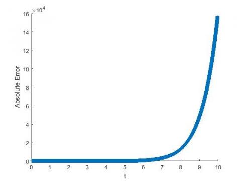
The follow Figure 1, show the absolute error between the exact and approximate solution of given IVPs by executing DTM: the absolute error is defined by
AbsoluteError$=\left|y-y_{s}\right|$
Figure 1. Magnitude of the absolute error
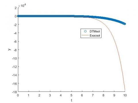
The following Figure 2, gives a graphical representation of the exact solution and the DTM approximate solution.
Figure 2. Comparison between the exact and DTM solutions
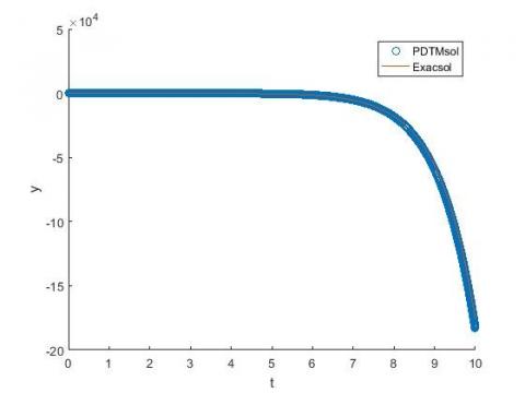
And Figure 3, gives a graphical representation of the exact solution and the PDTM approximate solution when
[0,T]=[0,10]=[0,1]∪[1,2]∪…∪[9,10]
Figure 3. Comparison between the exact and PDTM solution
Example 2:
$y^{\prime \prime}+2 y^{\prime}+y=e^{-t}, y(0)=-1, y^{\prime}(0)=1$
The exact solution of the above problem is
$y(t)=\left(\frac{1}{2} t^{2}-1\right) e^{-t}$
Applying DTM to the given problem, we have the recursive relation:
$Y(k+2)=\frac{1}{(k+1)(k+2)}\left(\frac{(-1)^{k}}{k !}-2(k+1) Y(k+1)-Y(K)\right)$
Using the above relation and initial values
$Y(2)=0, Y(3)=-\frac{1}{3}, Y(4)=\frac{1}{4}$
Using Eq. (3) the solution has been obtained as
$y(t)=-1+t-\frac{1}{3} t^{3}+\frac{1}{4} t^{4}-\frac{2}{15} t^{5}+\cdots$
Table 2. The numerical results of the exact solution and their approximations by using DTM and PDTM
|
t |
Exact value |
DTM value |
PDTM value |
|
0.1 |
-0.9003 |
-0.9003 |
-0.9003 |
|
0.5 |
-0.5307 |
-0.5312 |
-0.5307 |
|
1 |
-0.1839 |
-0.2833 |
-0.1833 |
|
5 |
0.0775 |
-1.1314e+03 |
0.0779 |
|
10 |
0.0022 |
-3.7824e+04 |
0.0027 |
Example 3: Consider the following integro-differential equation
$\begin{aligned} y^{\prime \prime}(t)=y^{\prime}(t)-1-\sin t \int_{0}^{t} y(x) d x \\\underline{\mathrm{y}}(0)=0, \mathrm{y}^{\prime}(0)=1\end{aligned}$
The analytical solution of the above problem is y(t)=sin t.
At t=0, we can find another initial condition as y'' (0)=0.
From the initial values we have Y(0)=0, Y(1)=1, Y(2)=0 and application of DTM yields the recursive relation:
$\begin{aligned} Y(k+2)=\frac{1}{(k+1)(k+2)} &[(k+1) Y(k+1)+\delta(k)-W(k)\\+& \frac{Y(k-1)}{k} ] \end{aligned}$
where $W(k)=\left\{\begin{array}{c}{0, \text { for } k \text { is even }} \\ {\frac{(-1)^{(k-1) / 2}}{k !}, \text { for } k \text { is odd }}\end{array}\right.$
Table 3. The numerical results of the exact solution and their approximations by using DTM and PDTM
|
t |
Exact value |
DTM value |
PDTM value |
|
0.0 |
0 |
0 |
0 |
|
π/10 |
0.19866 |
0.19866 |
0.19866 |
|
π/5 |
0.39841 |
0.39841 |
0.39841 |
|
π/2 |
1.0 |
1.0 |
1.0 |
|
π |
0 |
-0.01738 |
0.0 |
Example 4: Consider the following system of differential equations of order two:
$\left\{\begin{array}{c}{y_{1}^{\prime \prime}+y_{1}-y_{2}^{\prime \prime}-4 y_{2}=0} \\ {y_{1}^{\prime}+y_{2}^{\prime}=\cos 2+2 \cos 2 t}\end{array}\right.$
with the conditions
$\left\{\begin{array}{l}{y_{1}(0)=0, y_{1}^{\prime}(0)=1} \\ {y_{2}(0)=0, y_{2}^{\prime}(0)=2}\end{array}\right.$
The exact solution of this problem is
y(t)=(y_1 (t),y_2 (t))=(sin t,sin 2t )
By using the initial conditions
Y1(0)=0, Y1(1)=1, Y2(0)=0, Y2(1)=2
and application of DTM yields the recursive relation:
$\left\{\begin{array}{c}{(k+2)(k+1) Y_{1}(k+2)+Y_{1}(k)} \\ {-(k+2)(k+1) Y_{2}(k+2)-Y_{2}(k)=0} \\ {(k+1) Y_{1}(k+1)+(k+1) Y_{2}(k+1) |} \\ {=\frac{1}{k !} \cos \frac{k \pi}{2}+\frac{2^{k+1}}{k !} \cos \frac{k \pi}{2}}\end{array}\right.$
Consequently, we find
$\left\{\begin{array}{c}{y_{1}(t)=t-\frac{1}{3 !} t^{3}+\frac{1}{5 !} t^{5}+\cdots=\sin t} \\ {y_{2}(t)=2 t-\frac{8}{3 !} t^{3}+\frac{32}{5 !} t^{5}+\cdots=\sin 2 t}\end{array}\right.$
Table 4. Comparison of the numerical results with exact solution and absolute error (max between y1 error and y2 error)
|
t |
Exact value |
DTM error |
PDTM error |
|
0.1 |
(0.0017,0.0035) |
2.5443E−3 |
2.5443E−3 |
|
0.5 |
(0.0087,0.0174) |
1.9556E−3 |
1.9556E−3 |
|
1 |
(0.0174,0.0349) |
1.5629E−2 |
2.3793E−3 |
|
5 |
(0.0871,0.1736) |
3.0001E+1 |
1.7539E−2 |
|
10 |
(0.1736,0.3420) |
0.9015E+5 |
1.0417E−2 |
3.2 Discussions
As mentioned in Eqns. (4)-(8), the concept of DTM is derived from Taylor series expansion and the convergence of the method was studied in many works for small interval. If t1=T, then the partitioning DTM and the standard DTM are the same. However, when interval becomes large, this method gives the bad results or fail.
In Example 1, we show that for t>2 (see Figure 1,2), the absolute error between DTM and the exact solution increases as t increases. In Fig3, using the partitioning DTM, we can show that for large interval the application of DTM in each sub-interval gives a good accuracy.
In Example 2, the remark, that for t>1, the partitioning DTM method is used to improve the basic DTM in order to obtain a good approximations.
In example 3 and 4, we give the comparison between the exact value and the partitioning DTM value see Table 4 and 5.
The model of the transmissions powers electrical circuit is shown in paper [4]: ‘Solving differential equations analytically is difficult and tedious, especially when the equations are complicated and coupled’. In this section, we concentrate our effort to give an analytical approximation for solving the equations governing system.
First, we consider the examples discussed in [5] without equation differentiation and apply the PDTM approach to solve the electrical circuit problems that govern the Kirchhoff voltage laws as follow:
$L i^{\prime}+R i+\frac{1}{C} \int i d t=e(t)$ (11)
where e(t) the electromotive force, e0= constant, L inductance, R resistance, C capacitance and i(t) the instantaneous current.
The analytical approximation of (11) for k≥1 is given by
$I(k+1)=\frac{1}{L(k+1)}\left(E(k)-R I(k)+\frac{1}{C} \frac{I(k-1)}{k}\right)$
Using Eqns. (8)-(10), we have:
$\forall j \in\{0, \ldots, M-1\}$ and $[0, T]=U_{j=0}^{M-1}\left[t_{j}, t_{j+1}\right]$ and for all $t\in [0,T]$,
$\left\{\begin{array}{c}{i(t)=\sum_{j=0}^{M-1} i_{j}(t) \chi_{\left[t_{j} t_{j+1}\right]}(t)} \\ {i_{j}(t)=\sum_{l=0}^{N} I(k)\left(t-t_{j-1}\right)^{k}, t \in\left[t_{j-1}, t_{j}\right]}\end{array}\right.$
Example 5: [5]
$i^{\prime}+4 i+3 \int i d t=-2.25 \cos 2 t,$ with $i(0)=i^{\prime}(0)=0$
The exact to the problem is:
$i(t)=-\frac{9}{26} e^{-3 t}+\frac{117}{130} e^{-t}-\frac{72}{130} \cos 2 t-\frac{9}{130} \sin 2 t$
Applying DTM with I(0) = I(1) = 0 and the recursive relation
$I(k+1)=\frac{1}{k+1}\left(-4 I(k)-3 \frac{I(k-1)}{k}-2.25 \frac{2^{k}}{k !} \cos \frac{k \pi}{2}\right)$
In order to get the recursive relation given in [5] (Example 4), a simple change of variable k by k’+1 gives the result. The given IVP has the solution
$i(t)=\frac{3}{2} t^{3}-\frac{3}{2} t^{4}+\frac{27}{40} t^{5}-\frac{3}{10} t^{6}+\cdots$
Table 5. Comparison of the numerical results with exact solution with PDTM
|
T |
Exact value |
PDTM |
Absolute error |
|
0.1 |
0.00135646 |
0.00135646 |
1E-16 |
|
0.2 |
0.0097986 |
0.0097987 |
1.584E-8 |
|
1 |
0.48138748 |
0.5267857 |
4.54E-2 |
|
2 |
0.53535575 |
0.5395137 |
4.2E-3 |
|
3 |
-0.46767683 |
-0.47955 |
1.19E-3 |
As in [4], let consider the general electrical circuit defined in Figure 4, as follow:
The equations obtained by applying the Kirchhoff’s Voltage Law (KVL) in an electrical circuit consisting of two loops, namely:
$\left\{\begin{array}{c}{v_{1}=R_{1} i_{1}+L_{11} i_{1}^{\prime}-M_{12} i_{2}^{\prime}} \\ {v_{2}=R_{2} i_{2}+L_{22} i_{2}^{\prime}-M_{21} i_{1}^{\prime}+\frac{1}{C} \int i_{2} d t}\end{array}\right.$ (12)
where v1, v2: voltage,
i1, i2:current,
R1, R2: voltage,
L11, L22:self-inductance,
M12, M21:mutual inductance,
C: capacitance.
The coefficients associated with the proportional, differential and integral terms can be represented by resistance, inductance and capacitance, respectively.
In the calculation, it is assumed that:
$\left\{\begin{array}{c}{L_{11}=1, L_{22}=1} \\ {M_{12}=0.995, M_{21}=0.995} \\ {R_{1}=0.111, R_{2}=0.987247} \\ {C=0.111278} \\ {i_{1}(0)=0, i_{2}(0)=0} \\ {v_{C}(0)=0, v_{1}=10, v_{2}=0.0}\end{array}\right.$
with the capacitor voltage vc at time t=0 are zero.
By using the initial conditions and application of DTM yields the recursive relation:
$\left\{\begin{aligned} v_{1} \delta(k)=R_{1} I_{1}(k) &+L_{11} I_{1}(k+1)-M_{12} I_{2}(k+1) \\ v_{2} \delta(k)=R_{2} I_{2}(k) &+L_{22} I_{2}(k+1)-M_{21} I_{1}(k+1) \\ &+\frac{1}{C} \frac{I_{2}(k-1)}{k} \end{aligned}\right.$
Then,
$\left(\begin{array}{cc}{L_{11}} & {-M_{12}} \\ {-M_{21}} & {L_{22}}\end{array}\right)\left(\begin{array}{c}{I_{1}(k+1)} \\ {I_{2}(k+1)}\end{array}\right)=\left(\left(\begin{array}{cc}{v_{1} \delta(k)} \\ {v_{2} \delta(k)}\end{array}\right)-\left(\begin{array}{cc}{R_{1}} & {0} \\ {0} & {R_{2}}\end{array}\right)\left(\begin{array}{c}{I_{1}(k)} \\ {I_{2}(k)}\end{array}\right)\right)-\left(\begin{array}{c}{0} \\ {\frac{1}{C} \frac{I_{2}(k-1)}{k}}\end{array}\right)$
For k=0, we have
$\left(\begin{array}{c}{I_{1}(1)} \\ {I_{2}(1)}\end{array}\right)=\left(\begin{array}{cc}{L_{11}} & {-M_{12}} \\ {-M_{21}} & {L_{22}}\end{array}\right)^{-1}\left(\left(\begin{array}{c}{v_{1}} \\ {v_{2}}\end{array}\right)-\left(\begin{array}{cc}{R_{1}} & {0} \\ {0} & {R_{2}}\end{array}\right)\left(\begin{array}{c}{I_{1}(0)} \\ {I_{2}(0)}\end{array}\right)-\left(\begin{array}{c}{0} \\ {0}\end{array}\right)\right)=\left(\begin{array}{c}{1.0025 E+03} \\ {-0.9957 E+03}\end{array}\right)$
And for k≥1
$\begin{aligned}\left(\begin{array}{c}{I_{1}(k+1)} \\ {I_{2}(k+1)}\end{array}\right)=-\left(\begin{array}{cc}{L_{11}} & {-M_{12}} \\ {-M_{21}} & {L_{22}}\end{array}\right)^{-1}\left[\left(\begin{array}{cc}{R_{1}} & {0} \\ {0} & {R_{2}}\end{array}\right)\left(\begin{array}{c}{I_{1}(k)} \\ {I_{2}(k)}\end{array}\right)\right.\\ &+\left(\begin{array}{cc}{0} \\ {\frac{1}{C} \frac{I_{2}(k-1)}{k} )}\end{array}\right] \\ &=-\left(\begin{array}{cc}{L_{11}} & {-M_{12}} \\ {-M_{21}} & {L_{22}}\end{array}\right)^{-1}\left(\begin{array}{c}{R_{1} I_{2}(k)} \\ {R_{2} I_{2}(k)+\frac{1}{C} \frac{I_{2}(k-1)}{k}}\end{array}\right) \end{aligned}$
Let ∆=L11 L22-M12 M21, then
$\begin{aligned} I_{1}(k+1)=-\frac{1}{\Delta}( & L_{22} R_{1} I_{1}(k)+M_{12} R_{2} I_{2}(k) \\+\frac{M_{12}}{C} \frac{I_{2}(k-1)}{k} ) \\ I_{2}(k+1)=-\frac{1}{\Delta}( & M_{21} R_{1} I_{1}(k)+L_{11} R_{2} I_{2}(k) \\+\frac{L_{11}}{C} \frac{I_{2}(k-1)}{k} ) \end{aligned}$
Using the recursive relation and the Eq. (8), we obtain
$\left\{\begin{aligned} i_{1, m}(t)=& \sum_{k=0}^{n} I_{1, m}(k)\left(t-t_{m-1}\right)^{k} \\ i_{2, m}(t)=& \sum_{k=0}^{n} I_{2, m}(k)\left(t-t_{m-1}\right)^{k} \end{aligned}\right.$ for t∈[tm-1,tm] (13)
And
$\forall j \in\{0, \ldots, M-1\}$ and $[0, T]=\cup_{i=0}^{M-1}\left[t_{j}, t_{j+1}\right]$ and for all $t\in[0,T]$, we have
$\left\{\begin{aligned} i_{1}(t) &=\sum_{j=0}^{M-1} i_{1, j}(t) \chi_{\left[t_{j}, t_{j+1}\right]}(t) \\ i_{2}(t) &=\sum_{j=0}^{M-1} i_{2, j}(t) \chi_{\left[t_{j}, t_{j+1}\right]}(t) \end{aligned}\right.$ (14)
For the numerical results, we compare the proposed method to the analytical approximation given in [4] by:
$i_{2}(t)=-0.100858 e^{-0.1 t}+11.1952161 e^{-10 t}-11.094358 e^{-100 t} A$
And for comparison purposes, the numerical method mentioned above are tested with different time steps 0.001s, 0.01s, 0.02s and 0.03s in computation and with order 5.
Table 6. Comparison of the numerical results with reference solution [4] with different time steps T
|
T |
Reference value |
PDTM |
Absolute error |
|
0.001 |
0.9533093 |
0.9035725 |
0.0497 |
|
0.005 |
3.8475817 |
3.796201 |
0.0514 |
|
0.01 |
5.9781937 |
5.9386937 |
0.0395 |
|
0.02 |
7.5751726 |
7.5345726 |
0.0406 |
|
0.03 |
7.6321926 |
7.5820926 |
0.0501 |
In this work, we presented a new approach for applying the partitioning differential transform method for solving nonlinear integro-differential equations for large time interval. In Example 1, we show the effectiveness of this method when the classical differential transform method fail or give the bad results. The analytical approximations to the solutions are reliable, and confirm the power and ability of the partitioning DTM methods as an easy device for computing the solution of a non-linear system of differential or intergo-differential equations. For the considered test, the presented technique generated numerical results and is effective in solving nonlinear integro-differential equations.
The authors thank the referees very much for their constructive suggestions, helpful comments and fast response, which led to significant improvement of the original manuscript of this paper.
[1] Abdel-Halim Hassan IH. (2004). Differential transformation technique for solving higher-order initial value problems. Appl. Math. Comput. 154: 299-311. https://doi.org/10.1016/S0096-3003(03)00708-2
[2] Abdel-Halim Hassan IH. (2008). Application to differential transformation method for solving systems of differential equations. Applied Mathematical Modelling 32(12): 2552-2559. https://doi.org/10.1016/j.apm.2007.09.025
[3] Arikoglu A, Ozkol I. (2008). Solution of integral and integro-differential equation systems by using differential transform method. Comput. Math. Appl. 65: 2411-2417. https://doi.org/10.1016/j.camwa.2008.05.017
[4] Hui SYR, Christopoulos C. (1991). Discrete transform technique for solving coupled integro-differential equations in digital computers. In IEE Proceedings A - Science, Measurement and Technology 138(5): 273-280. https://doi.org/10.1049/ip-a-3.1991.0039
[5] Mohanty M, Jena SR. (2018). Differential transformation method (DTM) for approximate solution of ordinary differential equation (ODE). Advances in Modelling and Analysis B 61(3): 135-138 https://doi.org/10.18280/ama_b.610305
[6] Odibat ZM. (2008). Differential transform method for solving volterra integral equation with separable kernels. Math. and Comput. Model. 48: 1144-1149. https://doi.org/10.1016/j.mcm.2007.12.022
[7] Odibat ZM, Bertelle C, Aziz-Alaoui MA, Duchamp GHE. (2010). A multi-step differential transform method and application to non-chaotic or chaotic systems. Computers and Mathematics with Applications 59(4): 1462-1472. https://doi.org/10.1016/j.camwa.2009.11.005
[8] Evg. Pukhov G. (1982). Differential transforms and circuit theory. Circuit Theory and Applications 10: 265-276. https://doi.org/10.1002/cta.4490100307
[9] Zhou JK. (1986). Differential transformation and its application for electrical circuits. Huarjung University Press, Wu-uhahn, China.