Mohamed Kadri | Ahmed Sahli* | Sara Sahli
OPEN ACCESS
The present paper deals with the analysis of cylindrical shells by the application of the Weighed Residual Method, more specifically the Least Squared Method, to obtain approximate solutions of shells structural problems, especially the cylindrical reservoirs subjected to hydrostatic shipment in the linear behavior regime. The ways of obtaining the approximate solutions refer to the adoption of linear, polynomial approximate bases, as well as the possibility of enriching the approximation by adding functions with similar characteristics to the accurate solution itself. Such procedures can be useful in the analysis of structures to significantly prevent the rise of the computational effort, by means of an approximate base that corresponds to the characteristics required by the analytical solution of the problem.
container, cylindrical shells, enrichment, linear behavior, weighted residual method
Computational mechanics with its various numerical methods is being used to analyze different problems with various kinds of boundary conditions. Basically, the main advantage of meshless methods is to eliminate model meshing stage and to distribute nodal points throughout the model domain instead of meshing. In the element free Galerkin method (EFGM) using moving least squares (MLS) approximation, a linear combination of basic functions is fit to data by a weighted function [1].
The weighted residues method and its derived processes constitute formulations, which provide the obtainment of sufficiently accurate approximate solutions of a boundary value problem. They are expressed in a general form, weighted integration by the own representative differential equation of problem.
Bin Liang et al. [2] analyze two types of optimization of thin-walled cylindrical shells loaded by lateral pressure, with arbitrary axisymmetric boundary conditions and the volume being constant. The first is to find the optimal thickness to minimize the maximum deflection of a cylindrical shell. Here expressions of the objective function are obtained by the stepped reduction method.
A weighted Runge-Kutta discontinuous Galerkin method for the wave field modeling, which is simply called the WRKDG method, is developed by [3]. For this method, they first transform the seismic wave equations into a first-order hyperbolic system, and then combine the discontinuous Galerkin spatial discretization with a weighted Runge-Kutta time discretization.
Reference [4] presents a comparison of a reliability technique that employs a Fourier series representation of random axisymmetric and asymmetric imperfections in a cylindrical pressure vessel subjected to an axial end load and external pressure, with evaluations prescribed by the ASME boiler and pressure vessel code, section VIII, division 2 rules.
The paper of Gurinder et al. [5] contains a stress analysis of a cylindrical pressure vessel loaded by axial and transverse forces on the free end of a nozzle. The nozzle is placed such that the axis of the nozzle does not cross that of the cylindrical shell.
Classical simple formulae for elastic hoop stresses in cylindrical and spherical pressure vessels continue to be used in structural analysis today because they facilitate design procedures. Traditionally such formulae are only applied to thin-walled pressure vessels under internal pressure. There do exist, however, some variations of these formulae that remain simple yet permit wider use [6].
The problem of crack detection in cylindrical shell structures is investigated by [7]. To do this, the differential quadrature method and bees algorithm have been used.
In their study [8], static and free vibration characteristics of anisotropic laminated cylindrical shell with various end conditions are considered by making the use of differential quadrature method (DQM). Equations of motion are derived based on three-dimensional theory of elasticity.
Three-dimensional thermo-elastic analysis of a functionally graded cylindrical shell with piezoelectric layers under the effect of asymmetric thermo-electro-mechanical loads is carried out by [9]. Numerical results of displacement, stress and thermal fields are obtained using two versions of the differential quadrature methods, namely polynomial and Fourier quadrature methods.
An approach for simulating coupled acousto-elastic wave phenomena, including fluid-solid boundaries where the solid is allowed to be anisotropic, with the discontinuous Galerkin method, is developed by [10].
Regarding the shell structures, due to the specific characteristics of their differential equations, conventional numerical solution processes employing polynomial approximations can have a very significant degree of difficulty. Therefore, weighted residues methods combined with unconventional techniques for enriching the approximate function, can constitute effective alternative to reduce the degree of difficulty in solving the problem. However, polynomial functions are not always the most efficient for the initial approach enrichment purposes, notably the problems of shell structures. Usually analytical solutions have characteristics such that they can only be played through the adoption of a very high degree polynomial for enrichment, which implies high computational cost. Thus, recourse to the use of special functions not polynomial for enrichment can prevent, significantly, the increase in computational effort in structural analysis.
The present work has the objective of evaluating the performance of approximate solutions obtained by the application of Weighted Residues Methods, specifically the Galerkin Method and the Least Squares Method, to the analysis of structures of tubes submitted to hydrostatic loading.
Regarding the methods adopted for the development of the research, the strong forms and weighted residues with which boundary value problem is expressed are analyzed. A comparative study of approximate solutions obtained by the use of bases of linear and polynomial functions of higher degree for the generation of the approximation function, as well as of special functions that have the same characteristics of the analytical solution is developed.
The use of the enrichment technique of the approximate function on the form in weighted residues is also explored. Finally, the Finite Element Method for the approximation generation [11] for a boundary value problem formulated by the Least Squares Method is applied. In this sense, the work presents original contributions, such as the combination of approximation enrichment techniques on Weighted Residues Methods, and the application of the Least Squares Method with division of the integration domain, to solve the problem of linear behavior pipes.
2.1 Pipes with axisymmetric loading
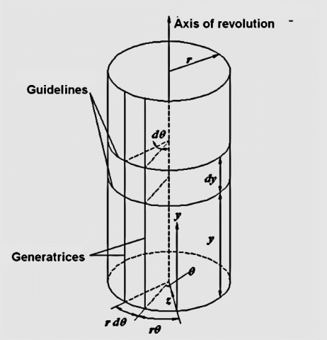
The shells are structural elements laminar and have an average surface not flat. This definition covers various structural shapes, said shell being revolution when its geometrical shape can be generated by rotating a line about an axis known as axis of revolution. In this work are considered, among the revolution shells, tubes, whose main geometric elements, with reference to their average surface are shown in Figure 1.
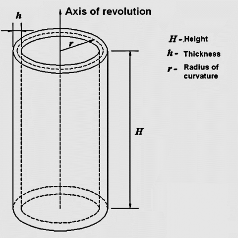
Among its geometric elements, also highlight the height H, the thickness h and the radius of curvature r of their average area indicated in figure 2.
In addition to internal pressure, circular cylindrical shell structures are often subject to concentrated or localized bending moments and forces of varying nature (external loads, loads arising from the interaction between structural components of differing stiffness, loads due to constraint reactions, and so forth), distributed symmetrically around the rotational axis [12-13].
Given our concern with conceptual design, we will use analytical models of general validity that, by introducing simplifying assumptions, ensure that the real world problem can be more readily addressed but in any case guarantee that the results thus obtained are meaningful in actual applications. Essentially, two simplifying assumptions will be introduced: axial symmetry in the broad sense (generalized axisymmetry), i.e., referring not only to the cylindrical body’s geometrical shape, but also to the surface forces (pressures) and the thermal load acting on it, its boundary conditions and the material’s elastic properties, and the assumption regarding the stress state and strain state [14-18]
Figure 1. Cylindrical tube
Figure 2. Geometric parameters of the revolution shell
With regard to external forces, it is considered only the work of a pressure Internal representing the action of a fluid contained by the tube, the latter being completely full (figure 3), given by the following equation:
$P=-γ(H-y)$ (1)
In these conditions the tube is characterized as a cylindrical reservoir.
Taking a generic element of the average surface, delimited by two generators and two guidelines, as Figure 1, indicate the internal forces arising from the action of the liquid pressure in the reservoir in Figure 4, whose variations are consistent with restrictions of geometric symmetry and axial loading. As we know from the standard texts [19-25], in the most general non-axisymmetric conditions, the small element of the circular cylindrical shell is subject to ten stress resultants per unit length, four in-plane (Ny; Nq; Nyq ; Nqy) and six out-of-plane (Ty; Tq; My; Mq; Myq; Mqy). The in-plane stress resultants are also termed membrane stress resultants. Imposing equilibrium conditions, it can be inferred that, as a result of axisymmetry, the membrane shearing forces Nyq and Nqy must be zero (Nyq = Nqy = 0), the transverse shearing forces Tq acting on the sides of length dz must be zero (Tq = 0) and the twisting moments Myq and Mqy must also be zero (Myq = Mqy = 0). As five out of the ten stress resultants are thus zero, viz., Nyq, Nqy, Tq , Myq , Mqy; they are not shown in Figure 4.
Figure 3. Hydrostatic pressure in the cylindrical reservoir
Figure 4. Applicants efforts in the cylindrical reservoir
Imposing the static equilibrium of forces and moments in the generic shell element, according to the directions defined by the axes x, y and z, result, the following equilibrium relationships:
$-\frac{dM_y}{dy}+Q_y=0$ (2a)
$\frac{(dN_y}{dy}+P_y=0$ (2b)
$r\frac{dQ_y}{dy}+N_θ+P_z.r=0$ (2c)
By combining the Eq. (2.3a) and Eq. (2.3c), we obtain:
$r \frac{d^2 M_y}{(dy^2}+N_θ+P_z.r=0 $ (3)
Note that Eq. (2b) refers to the equilibrium relative to the wall own weight, which is independent of the other equation Eq. (2a) and Eq. (2c). In the case where the bending moment throughout their height is null, by Eq. (3) are obtained:
$N_θ=-P_z.r $ (4)
In this case, note that the displacement of the vessel wall can be determined by the radius length variation of the reservoir, Eq. (7). In view of Eq. (4), Eq. (5), and Eq. (6) mentioned below:
$ε_θ=\frac{σ_θ}{E}$ (5)
$σ_θ=\frac{N_θ}{h}$ (6)
The displacement function:
$w(r)=∆r=-ε_θr=-(\frac{σ_θ}{E})r=-\frac{r}{E}(\frac{N_θ}{h})=-N_θ\frac{r}{Eh}$ (7)
Thus, the rotation of the wall of the reservoir can be expressed by the first derivative of the displacement function:
$\frac{dw(y)}{dy}=\frac{γr^2}{Eh}$ (8)
In view of Eq. (2a) and Eq. (2c) which define the bending problem in cylindrical walls shells, they are two equations and three unknowns: Nθ, My and Qy. In this case, you must enter a relationship between forces and displacements, because the problem is internally hyperstatic. This relationship can be obtained from Eq. (7):
$w(r)=∆r=-ε_θr=-(\frac{σ_θ}{E})r=-\frac{r}{E}(\frac{N_θ}{h})=-N_θ\frac{r}{Eh}$
so that:
$w(r)=-N_θ\frac{r}{Eh}$ →$N_θ=-\frac{Eh}{r}w(r)$ (9)
With this, Eq. (2c) may be described as follows:
$r\frac{dQ_y}{dy}-\frac{Eh}{r}w+P_z.r=0$ (10)
The third problem is the equation given by:
$M_y=-D\frac{d^2w}{(dy^2}$ (11)
Thus, there is now a problem with three equations: Eq. (2), Eq. (10) and Eq. (11). And three unknowns (Nθ, My and Qy) that can be reduced to two equations: Eq. (11) and Eq. (12). And two unknowns (Nθ and My):
$r\frac{d^2M_y}{dy^2}-\frac{Eh}{r}w+P_z.r=0$ (12)
Substituting Eq. (11) in Eq. (12), we obtain the equation that describes the behavior of cylindrical walls subjected to hydrostatic pressure, Eq. (13):
$r\frac{d^2}{dy^2}(-D\frac{d^2w}{dy^2})-\frac{Eh}{r}w+P_z.r=0$
$D\frac{d^4 w}{dy^4}+\frac{Eh}{r^2}w=P_z$ (13)
Or yet:
$\frac{d^4w}{dy^4}+4β^4w-\frac{P_z}{D}=0$ (14)
Where:
$β=∜\frac{3(1-ϑ^2)}{(h^2r^2}$; $D=\frac{Eh^3}{12(1-ϑ^2)}$ (15)
Once obtained the displacement w by solving the differential equation (2.14) can be determined all the parameters that characterize the static regime of the shell.
The general solution of Eq. (14) is given by the following equation:
$w=e^{βy}(C_1 cos(βy)+C_2 sin(βy))+e^{-βy}(C_3 cos(βy)+C_4 sin(βy))+f(y) $ (16)
where f (y) is a particular solution of the problem. In the case of pressure Hydrostatic, the particular solution of this equation is given by:
$f(y)=(\frac{r^2}{Eh})P_z=(\frac{γr^2}{Eh}(H-y)$ (17)
The constant appearing in Eq. (16) should be obtained from the imposition of boundary conditions. In this paper, for simplicity, we consider only cases of reservoir with hinged fixed and cantilever base, both with free top (zero bending moment and shear).
3.1 Enrichment approach
The method of weighted residues establishes a natural condition for obtaining approximate solutions to many engineering problems. According Assan [26], the method of weighted residues differs from the so-called variational methods per no need the existence of a functional, directly using the differential equation (strongly) of the problem to be solved.
In order to improve the quality of approximation, one can opt for use of an enrichment technique, which consists in expanding the basis of approximate functions already existing. The enrichment can be performed by direct addition of whole new basis functions existing, or by adding new terms resulting from the base multiplied by the previous base, when constitutes a unit of partition [27]. This paper presents the second enrichment option, under the meshless methods. Just like further remark such methods generate approaches from local functions defined in each nodal point hitching to it a local domain of influence called cloud, [27].
3.2 Method of weighted residuals with enrichment for the tubes problem
Considering the approximate representation of functions of the method weighted residual according to equation:
$\check{u}(x)=α_i∅_i(x)+\check{u_0}(x)$ $i=1,…,n$ (18)
where $\check{u}(x)$ is the function that satisfies the constraints essential and natural contour, $∅_i(x)$ are homogeneous functions in those restrictions, $α_i$ are the unknown parameters of the problem.
The enrichment technique is to introduce a basis functions $φ_k$, said enriching, so that the new basis for the approximation $\check{u_e}$ result:
$\check{u_e}(x)=α_i.∅_i(x)+λ_ik.∅_i(x).φ_k+\check{u_0}(x)$ $i=1,…..n$ $k=1,……p$ (19)
where p is the number of terms in the new base. Of course, the approximate solution should check the conditions of essential and natural contour. By definition, it follows that the residue of approximation is given by the following equation:
$R(\check{u_e})=A(\check{u_e})-f$ (20)
where A is a differential operator of the function u (exact solution), responsible for generating plots containing different orders of derivatives that may appear on a specific problem.
Annulment this residue in weighted form it is a condition for determining the coefficients of the approximate solution as follows:
$\sum_ΩR(\check{u_e}).Ψ_jdΩ=0$ (21)
where Y is the weight function (a base functions linearly independent).
The Eq. (21) generates the linear system, which defines the constants of approximate solution:
$α_i.A_ij=f_j$
The method of weighted residues states that the $α_i$ coefficients contained in the approximate function are determined by the condition of residue annulment in shape weighted in the field of solution.
Reuniting the coefficients in a column vector α, the coefficients $f_j$ into another column vector f and the coefficients $A_{ij}$ in line positions i and j column of a matrix A.
Note that, the $α_i$ now indicate all the coefficients of Eq. (19).
One of the drawbacks presented by the technique refers to the cost computer which is required every time you enter an enriching role in the issue. If the linear system with non-enriched base is of size n × n, after the introduction of enriching function obtains a system with dimensions (p + 1) ⋅ n × (p + 1) ⋅ n, where p is the number of enriching functions.
4.2.1 Enrichment of linear polynomial basis with Exponential-trigonometric base
The analytical solution of the cylindrical tube, appear linear polynomial terms, that well represent the membrane behavior, and exponential terms that well represent the membrane behavior, and exponential-trigonometric terms, harvesting the effects of localized bending. These characteristics can be directly utilized in the generation of approximate functions.
Therefore, one can approximate function from a polynomial basis and apply the enrichment technique with auxiliary functions f1 and f2, of type:
$f_1=e^{-βy}.cos(βy)$ (22)
$f_2=e^{-βy}.sin(βy)$ (23)
More specifically, for a cylindrical vessel, articulated at the base and free at the top, considering the enrichment for functions f1 and f2 a linear function $\check{w}$ defined by equation (24).:
$\check{w}(y)=α_1.y+α_2$ (24)
Results in the following function enriched and :
$\check{w_e}(y)=α_1.y+α_2.y.e^{-βy}.cos(βy)+α_3.y.e^{-βy}.sin(βy)+α_4+α_5.e^{-βy}.cos(βy)+α_6.e^{-βy}.sin(βy)$ (25)
The problem of boundary conditions are as follows:
a) Essential boundary condition: displacement on the basis null
$\check{w_e}(0)=0$ (26)
b) Natural boundary condition: Bending Moment on the basis null
$\frac{d^2\check{w_e}(0)}{dy^2}=0$ (27)
So that when applying these conditions on enriched function results:
$\check{w_e}(y)=α_1.y+α_2.y.e^{-βy}.[cos(βy)+sin(βy)]+α_3[1-e^{-βy}]+α_4.e^{-βy}.sin(βy).(1+βy)$ (28)
Thus, the base enriched functions are defined as follows:
$∅_1=y$ (29)
$∅_2=y.e^{-βy}.[cos(βy)+sin(βy)]$ (30)
$∅_3=1-e^{-βy}$ (31)
$∅_3=e^{-βy}.sin(βy).(1+βy)$ (32)
Under these conditions the enriched approach, with the boundary conditions implied, can be represented as:
$\check{w_e}(y)=α_1.∅_1(y)+α_2.∅_2(y)+α_3.∅_3(y)+α_4.∅_4(y)$ (33)
Applying the definition of weighted residues method, coefficients can be determined by:
$α_i.\int_ΩA(ϕ_i ).Ψ_jdΩ=\int_Ωf.Ψ_j dΩ$ (34)
Recalling that the problem of cylindrical vessels differential operator $A(ϕ_i )$ and the function are given by:
$A(ϕ_i )=\frac{d^4 ϕ_i}{dy^4}+4.β^4.ϕ_i$ (35)
$f=\frac{P_z}{D}$ (36)
Since the equation (34), can be rewritten as follows:
$α_i.(\int_Ω\frac{d^4ϕ_i}{dy^4}.Ψ_j dΩ+4.β^4.\int_Ωϕ_i .Ψ_jdΩ)=\int_Ω\frac{P_z}{D}.Ψ_j dΩ$ (37)
Or implicitly represented as:
$α_i.A_{ij}=f_j$ (38)
In previous relationship, we have:
$A_{ij}=\int_Ω\frac{d^4ϕ_i}{dy^4}.Ψ_jdΩ+4.β^4.∫_Ωϕ_i .Ψ_jdΩ$ (39)
$f_j=\int_Ω\frac{P_z}{D}.Ψ_jdΩ$ (40)
A specific variant of weighted residues method that will be used, it is then dependent on the function to be adopted. In the following are shown the applications of Galerkin and least squares methods.
3.3 Method of Galerkin
The first example of this case, resolves the problem of a reservoir with an articulated base, imposing itself prior to approaching the essential boundary conditions at the base in relation to displacement and natural referring to the bending moment. The natural boundary conditions for the reservoir top are directly checked by the approach. In the graphs (Figures 5, 6 and 7) of displacement, bending moment and shear shown below, highlights the potential of the Galerkin method to capture exact solutions by adopting a basis for approximate function that contains the same solution characteristics.
Then they present the graphs of displacement, bending moment and shear:
Articulated base – Galerkin
Figure 5. Displacement obtained by the enrichment of the approximation
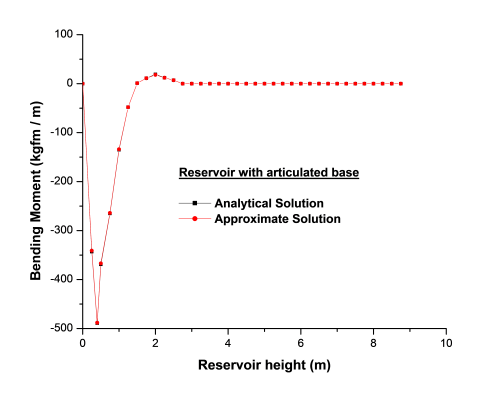
Figure 6. Bending Moment obtained by the enrichment of the approximation
Fixed base – Galerkin
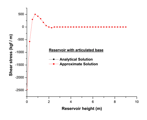
Figure 7. Shear stress obtained by the enrichment of the approximation
The second example of this case, resolves the problem of a reservoir with cantilever base, imposing previously the essential boundary conditions on the basis relative to the nullity of displacement and rotation. As in the case of articulated reservoir, it is evident that the potential of the Galerkin method to capture the exact solutions to adopt a base to approximate function that contains the same characteristics as the exact solution (Figures 8, 9 and 10).
The present Galerkin method can be seen to give very satisfactory results in comparison to analytic solution.
Figure 8. Displacement obtained by the enrichment of the approximation
Figure 9. Bending Moment obtained by enrichment of the approximation
Figure 10. Shear stress obtained by the enrichment of the approximation
3.4 Least Squares Method (LSM)
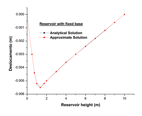
The same previous examples are now analyzed with the Least Squares process. As shown in the graphs of displacement, bending moment and shear, this method can also capture very specific solutions by using a basis for the approximation function that contains the same features as the exact solution. The results for Examples articulated and clamped reservoir are shown in the following Figures (11 - 16).
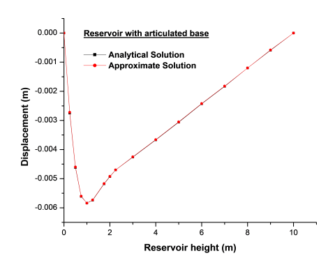
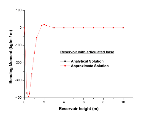
Articulated base – LSM
Figure 11. Displacement obtained by exponential-trigonometric approximation
Figure 12. Bending moment obtained by exponential-trigonometric approximation
Figure 13. Shear stress obtained by exponential-trigonometric approach
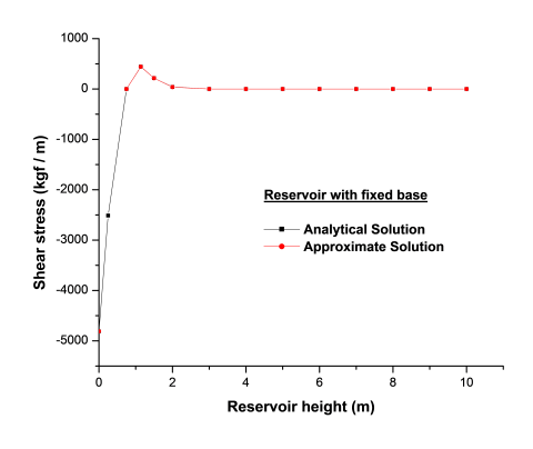
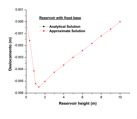
Fixed base – LSM
Figure 14. Displacement obtained by exponential-trigonometric approximation
The general principles of the forecasting estimation method are presented for indexes with different nature, this method is based on the least squares matrix. Among the advantages of the proposed method is the availability of explicit expressions for formula estimates saving structure of relations between the characteristics.
Figure 15. Bending Moment obtained by exponential-trigonometric approximation
Figure 16. Shear stress obtained by exponential-trigonometric approximation
In this research, apply formulations derived from the Weighed Residual Method in Resolution of reservoirs subjected to hydrostatic loading. The responses were analyzed using Galerkin methods and least squares, considering directly the weighted integral of the differential equation problem.
In both methods were adopted different approximate functions: bases polynomial, mixed bases composed of linear polynomial terms and terms Exponential-trigonometric. Regarding the polynomial based approximations generated with higher degree, it was found that the extent that it increases the polynomial of the degree approximately the response tends to exact answer. However, it is necessary to adopt very high degree of polynomial terms to achieve greater adherence to the exact solution. For this type of approach, comparing the methods, it was found that both presented very similar accuracy and computational effort.
As the use of mixed bases with functions having the same characteristics as the exact solution, firstly, it was not necessary to apply the natural boundary conditions related to the free top of the reservoir, because the exponential terms generate sufficient damping to reset the bending stresses along the height of the extended shells. In addition, in both methods, the approximate solution coincided with the exact solution, demonstrating the potential of methods to capture exact solutions by adopting an approximate base containing the same characteristics as the exact solution.
[1] Salari-Rad H, Rahimi Dizadji M. (2011). Meshless simulation of rock mechanics problems by element free Galerkin method. 12th ISRM Congress, 16-21 October, Beijing, China International Society for Rock Mechanics. ISRM-12CONGRESS-2011-083.
[2] Liang B, Noda N, Zhang SF. (2006). Two types of optimization of a cylindrical shell subjected to lateral pressure. International Journal of Pressure Vessels and Piping 83(7): 477–482. https://doi.org/10.1016/j.ijpvp.2006.04.001
[3] He XJ, Yang DH, Zhou YJ. (2014). A weighted Runge-Kutta discontinuous Galerkin method for wavefield modeling. SEG Annual Meeting, 26-31 October, Denver, Colorado, USA.
[4] Brar GS, Hari Y, Williams DK. (2013). Fourier series analysis of a cylindrical pressure vessel subjected to axial end load and external pressure. International Journal of Pressure Vessels and Piping 107: 27–37. https://doi.org/10.1016/j.ijpvp.2013.03.008
[5] Petrovic A. (2001). Stress analysis in cylindrical pressure vessels with loads applied to the free end of a nozzle. International Journal of Pressure Vessels and Piping 78(7): 485–493. https://doi.org/10.1016/j.ijpvp.2013.03.008
[6] Sinclair GB, Helms JE. (2015). A review of simple formulae for elastic hoop stresses in cylindrical and spherical pressure vessels: What can be used when. International Journal of Pressure Vessels and Piping 128: 1–7. http://dx.doi.org/10.1016/j.ijpvp.2015.01.006
[7] Moradi S, Tavaf V. (2013). Crack detection in circular cylindrical shells using differential quadrature method. International Journal of Pressure Vessels and Piping 111–112: 209–216. http://dx.doi.org/10.1016/j.ijpvp.2013.07.006
[8] Alibeigloo A. (2009). Static and vibration analysis of axi-symmetric angle-ply laminated cylindrical shell using state space differential quadrature method. International Journal of Pressure Vessels and Piping 86(11): 738–747. http://dx.doi.org/10.1016/j.ijpvp.2009.07.002
[9] Alashti AR, Khorsand M. (2011). Three-dimensional thermo-elastic analysis of a functionally graded cylindrical shell with piezoelectric layers by differential quadrature method. International Journal of Pressure Vessels and Piping 88(5-7): 167–180. http://dx.doi.org/10.1016/j.ijpvp.2011.06.001
[10] Ye RC, de Hoop MV. (2014). A 3D Discontinuous galerkin method for the propagation and scattering of acousto-elastic waves. SEG Annual Meeting, October, Denver, Colorado, USA, 26-31.
[11] Duarte CA, Babuŝka I, Oden JT. (2000). Generalized finite element methods for three dimensional structural mechanics problems. Computers & Structures 77(2): 215-232. http://dx.doi.org/10.1016/S0045-7949(99)00211-4
[12] Brownell LE, Young EH. (1968). Process equipment design. New York: Wiley.
[13] Jaward MH, Farr JR. (1989). Structural analysis and design of process equipment (2nd ed.). New York: Wiley.
[14] Vullo V. (2014). Circular cylinders and pressure vessels. springer series in solid and structural mechanics 3. Springer International Publishing, Switzerland. http://dx.doi.org/10.1007/978-3-319-00690-1_10
[15] Sokolnikoff IS. (1956). Mathematical theory of elasticity. New York: McGraw-Hill Book Company.
[16] Timoshenko SP, Goodier JN. (1970). Theory of elasticity (3rd ed.). New York: McGraw Hill.
[17] Boresi AP, Chong KP. (2000). Elasticity in engineering mechanics. New York: Wiley.
[18] Haupt P. (2000). continuum mechanics and theory of materials. Berlino: Springer.
[19] Timoshenko SP, Woinowsky-Krieger S. (1959). Theory of plates and shells (2nd ed.). Singapore: Mc Graw-hill Book Company.
[20] Tsui EYW. (1968). stresses in shells of revolution. Menlo park: Pacific cost publishers.
[21] Baker EH, Cappelli AP, Kovalevsky L, Rish FL, Verette RM. (1968). Shell analysis manual. North American Aviation, Inc., NASA CR-912, Washington, DC.
[22] Novozhilov VV. (1970). Thin shell theory (2nd ed.). Groningen: Wolters-Noordhoff Publishing.
[23] Cicala P. (1977). Asymptotic approach to linear shell theory. AIMETA Research Report, No. 6, p. 129.
[24] Flügge W. (1960). Stresses in shells (2nd ed.). Berlin: Springer (reprint of 1973).
[25] Ventsel E, Krauthammer T. (2001). Thin plates and shells: Theory, analysis, and applications. New York: Marcel Dekker Inc.
[26] ASSAN AE. (2003). Finite element method: First steps. 2.ed. Campinas: Publisher of Unicamp.
[27] Duarte CA, Oden JT. (1995). Hp Clouds – A Meshless method to solve boundary value problems. [S.1.], Technical report.