OPEN ACCESS
HVAC systems for controlled microclimate environments can be very energy consuming depending on the specific thermo-hygrometric conditions to be attained with respect to the conditions of external air. The aim of the present work is the analysis of some useful strategies devoted to reduce HVAC energy consumption. To this end, an in-house developed software is employed to evaluate energy consumption in terms of heating/cooling, humidification/dehumidification and reheat contributions. The test-case considered in this work is a museum environment where specific conditions are required to ensure long-term safety and preservation of the exhibitions by considering also visitors occupancy. The HVAC system is coupled with the exhibition room where the energy demand is computed through the microclimate energy balance. The simulation model has been validated by comparing the results in terms of energy demand to those obtained in the literature. Different strategies have been implemented to reduce the energy cost, i.e. a partial by-pass of cooling coil, an increase of the accepted tolerance for the relative humidity set-point value, an improvement of the thermal insulation of the building and a recirculation of the microclimate air. The results obtained by adopting such strategies have been compared to assess the efficiency of HVAC systems.
HVAC, energy efficiency, dynamic simulation
The conditioning process of controlled microclimate environments requires HVAC systems that are able to keep stable conditions of indoor air quality regardless of the outside conditions. Environments with strictly air quality requirements need a preliminary analysis of the actual energy performance concerning the building-plant system. Specifically, the present study is focused on the energy performance analysis applied to a museum environment. It is well known that, in such an environment, the control of the conditioning process is very important to allow the artwork conservation and to guarantee thermal comfort within the exhibition room. An interesting study concerning the monitoring of a museum environment is shown in [2], where an experimental method has been investigated based on field surveys in terms of both microclimate and microbiological requirements. The study highlights how the energy performance depends on the building envelope features, on the control strategy and on the management of HVAC system.
In [3], a methodology based on a medium/long-term monitoring provides a synthetic index to qualify the indoor air quality of a temporary exhibit. The methodology consists of three main steps: the analysis of HVAC features, the monitoring of significant thermal parameters and finally the energy consumptions analysis in order to provide a performance index as a measure of the energy behavior of the microclimate environment. The index takes into account both temperature and relative humidity changes. Within the room, these thermal-hygrometric parameters are the most important ones because affect the change of indoor microclimate as shown in [4]. Indeed, the study investigates the negative effects of the environmental parameters (relative humidity, indoor temperature and temperature of exhibits, improper lighting and atmospheric pollution) on the artworks conservation. The impact of temperature and relative humidity changes within exhibition rooms have been analogously studied in [5-7]. Specifically, the analysis performed in [5] refers to the Royal museum of fine arts (Belgium) and shows that, during the cold season, the building needs to be heated and the water vapor content of the mixture is very low compared to indoor relative humidity (RH). Therefore, a controlled conditioning process in terms of humidification and heating process is mandatory for the artworks conservation. Hence, the control strategy of HVAC system, which takes into account the well-being of visitors as priority, does not consider the optimal thermodynamic state for exposures. Furthermore, steady conditions should be preserved since effect of temperature and relative humidity variations is cumulative, and in the long run, this is detrimental to artefacts, as shown in [6]. Furthermore, the monitoring of indoor microclimate in terms of thermo-hygrometric conditions, air pollution, deposition and origin of the suspended particulate matter and microorganisms is necessary in order to qualify the conditioned environment [6]. The case study of [7] refers to the Correr Museum of Venice and the analysis is focused to identify malfunctions caused by the HVAC system. Moreover, the influence of the presence of carpets is also taken into account.
The control strategy of indoor relative humidity is mandatory in controlled microclimate to ensure the balance between the thermal load due to the occupants in exhibition areas and the latent load related to outdoor air humidity [8]. Analysis under different boundary conditions and control system HVAC has been carried out in [8-10]. Based on the same hourly climatic data source, the authors in [8] simulate a control system within a modern museum by using the dynamic simulation code DOE2.1. In [9], an in-house code has been developed for the analysis and optimization of energy systems used to control the environment microclimate, and in [10-11] two different HVAC control systems are implemented based on the predictive mathematical model given in [9]. The study of [11] investigates the energy behavior of controlled microclimate under different operating and climatic conditions by adopting different control system strategies. In [12], an analysis has been carried out to compare different suitable air diffusion equipments, in order to study the spatial distribution of thermo-hygrometric parameters. The case study is a modeled typical exhibition room.
Numerical codes based on Building Energy Performance Simulation (BEPS) and Computational Fluid Dynamic (CFD) techniques have been used to analyze the controlled microclimate environment. Innovative temperature and humidity independent control devices and control strategies are presented in [13], where the temperature and humidity parameters are conditioned independently on each other. The strategy control system can achieve independent temperature and humidity control in an energy saving way. The study shows that by employing this conditioning device, the energy consumption is reduced by 21.7 % compared with the conventional HVAC systems. An interesting energy performance study is shown in [14], where a detailed analysis is carried out in order to qualify the actual HVAC system for the case study. An integrated heat air and moisture model is developed and validated by a comparison with available numerical results and measurements. The study is focused on the development and validation of a dynamic simulation model based on actual energy consumption. Finally, an improvement of air conditioning plant is proposed to achieve a significant energy saving of the microclimate.
The aim of the present work is the analysis of some useful strategies devoted to reduce HVAC energy consumption in terms of heating/cooling, humidification/dehumidification and reheat contributions. The case study is a museum environment, where specific conditions are required to ensure long-term safety and preservation of the exhibitions, by including also visitors occupancy. The HVAC system is fully coupled with the exhibition room, where the energy demand is computed through the microclimate energy balance. The dynamic simulation model has been validated by comparing the thermal energy demand to that given in [1]. An all-air HVAC system with constant air volume for single zone is employed. The analysis is performed by selecting a seasonal set point with indoor air temperature gradually ranging from 21±1 °C to 23±1 °C. The comparison has been performed by evaluating the annual gas request for heating, humidification and reheat processes, whereas dehumidification and cooling contributions have been compared in terms of annual electrical energy request. In this work, several strategies have been implemented to reduce the energy cost, i.e. a partial by-pass of cooling coil, a recirculation of microclimate air, an increase of the accepted tolerance for the relative humidity set-point value and an improvement of the thermal insulation of the building. The results obtained with such strategies have been compared to assess the efficiency of HVAC systems. Several simulations are carried out in order to provide an exhaustive sensitivity analysis under different boundary conditions. Results are discussed in detail.
This work is organized as follows: first the main features of the simulation model are given, then the results are shown in terms of model validation and sensitivity analysis under different boundary conditions, and, finally, conclusions are summarized.
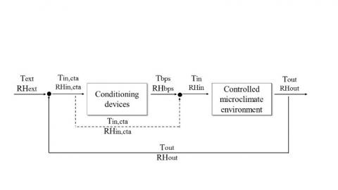
The simulation model analyses the thermodynamics of the conditioning processes of HVAC systems for controlled microclimates. As shown in Figure 1, the dynamic model consists of the following three main sections:
Figure 1. Structure of the simulation model
In the first section, the input conditions are selected. Specifically, the set-up conditions, in terms of temperature and relative humidity in the microclimate, the weather data set, in terms of hourly average values of outside air temperature and relative humidity, and the thermo-hygrometric conditions of the boundaries of the environment are given. In the second section, the HVAC is simulated and conditioning devices are defined. Specifically, the HVAC system adjusts the air humidity by increasing/decreasing the water content in the mixture when the absolute humidity is lower/greater than the humidity at the corresponding set-point temperature. Besides, the conditioning process changes the air temperature by heating/cooling the moist air in order to achieve the comfort conditions within the controlled environment.
Figure 2. Layout of the partial by-pass of cooling coil
A partial by-pass of cooling coil is implemented, as shown in Figure 2. This means that when cooling and dehumidification processes occur, the conditioning device cools only a fraction of the air. The temperature of the conditioned air at the exit of the cooling coil, named bypass temperature, is computed based on the temperature at the inlet and outlet of the cooling unit such that the temperature of the moist air obtained by mixing the bypass air and the conditioned moist air is equal to the set-point value, according to Eq.1:
$\mathrm{T}_{\mathrm{bps}}=\max \left(\frac{\mathrm{T}_{\mathrm{in}}-\mathrm{bps} \cdot \mathrm{T}_{\mathrm{in}, \mathrm{cta}}}{1-\mathrm{bps}}, 2\right)\left[^{\circ} \mathrm{C}\right]$ (1)
where:
Tbps is the bypass temperature [°C];
Tin is the temperature at the inlet of conditioned room [°C];
Tin,cta is the temperature at the inlet of cooling unit [°C];
bps is the fraction of air flow rate which does not have to be conditioned [-]. This parameter assumes values within the range 0÷1.
To avoid the water vapor changes to ice, a minimum value of Tbps is provided. This phenomenon can occur during the cooling process when the Tbps is lower than 2°C. By setting Tbps equal to 2°C, a new bps coefficient is calculated.
As concerns air humidity, the minimum/maximum value of vapor content in the mixture is evaluated by considering the range of comfort of relative humidity and the set-point temperature.
To improve the efficiency of HVAC system and ensure the comfort within the conditioned environment, a recirculation of the microclimate air is implemented. For each hour, the air flow rate to be conditioned at the inlet of the conditioning unit is obtained by mixing external air and recirculated air. In the model validation process, the recirculated air is equal to 21.3% of the total amount of air to be conditioned. Hence, the total conditioned air flow rate is assessed according to Eq. (2):
$\mathrm{G}=0.787 \cdot \mathrm{G}_{\mathrm{a}}+0.213 \cdot \mathrm{G}_{\mathrm{rec}}[\mathrm{kg} \cdot \mathrm{h}-1]$ (2)
where:
G is the total air flow rate to be conditioned [kg.h-1];
Ga is the external air flow rate [kg.h-1];
Grec is the recirculated air flow rate [kg.h-1].
When heating and humidification processes occur the whole air flow rate is conditioned, whereas in the other cases the conditioned air flow rate is a fraction of G based on bps.
At the beginning of the simulation, the model reads the input data, i.e. the climatic conditions in terms of temperature and humidity, the thermo-hygrometric parameters of surrounding environment, the set-point temperature and the range of comfort in terms of relative humidity and tolerance value. Based on these data-set, the model evaluates the temperature at the outlet of the conditioned environment based on the energy balance applied to the controlled environment. The energy balance is solved by assuming the following conditions:
At each time step, an iterative process has been implemented to estimate the vapor content in the mixture at the outlet of the room that will be used to determine the conditions at the inlet of the conditioning device due to the air recirculation. The block diagram of Figure 3 shows the steps of the iterative algorithm. At the beginning of the conditioning process, an initial guess for the outlet relative humidity is set to estimate the conditions at the inlet of CTA. Then, the relative humidity at the outlet of the room is compared to the new value computed at the end of the conditioning process. The optimal solution is reached when two subsequent iterations provide a tolerance (absolute value) of the outlet relative humidity lower than 10-6.
Figure 3. Sketch of the iterative algorithm
Finally, the dynamic model provides the energy consumption for each energy contributions: heating, humidification, cooling, dehumidification and reheat.
The case study deals with the analysis and optimization of HVAC systems for the conditioning of exhibition rooms. In order to validate the simulation model, the same museum of [1] is considered. The results of the simulation have been compared in terms of annual electric energy request as regards cooling and dehumidification, whereas the gas request has been compared for heating, humidification and reheat. The main features of the exhibition room are summarized in Table 1.
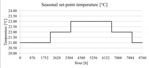
Figure 4 shows the seasonal set-point temperature selected in the simulation, which is equal to 21 °C during the cold months, 22 °C in the milder climate months and 23 °C during the summer season.
Figure 5 shows the comparison between the weather data (TRY [15]) employed in the model validation and the data used in [1]. The monthly averaged temperatures are very similar during the whole year, except for August. There are also some small differences in terms of monthly averaged relative humidity, especially in August. However, the diagrams show that the two databases follow a similar trend as regards both ambient temperature and relative humidity.
Table 1. Features of the exhibition room
|
Area |
272 m2 |
|
Volume |
1,360 m3 |
|
Indoor T |
seasonal set-point |
|
Indoor RH |
50 ± 5 % |
|
Outdoor climatic data |
Rome – TRY data |
|
Occupancy level design data |
0.3 person m-2 |
|
Occupant metabolic rate |
1.5 met person-1 |
Figure 4. Seasonal set-point temperature in the whole year
Figure 5. Comparison between TRY and Ref. [1] climatic data
In this section, the results of several simulations are presented and carefully discussed. The first subsection deals with the model validation. In the second subsection, the model is used to analyze the sensitivity of the results to different operating conditions, in order to study the performances of the whole energy system and improve its efficiency.
4.1 The model validation
In order to validate the model set-up, the evaluation of the energy request of the given test case has been carried out by considering the weather conditions of the city of Rome. The computations have been carried out by considering the specifics given in Table 1, i.e. a range 50 ± 5% for the relative humidity has been employed. A bps value equal to 0.5 is also selected.
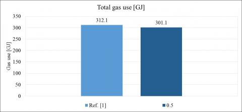
Figure 6 and Figure 7 show the comparison between the results obtained in this work and those of [1] in terms of energy consumption. Specifically, Figure 6 provides the gas request for heating, humidification and reheat, whereas Figure 7 gives the energy request for cooling and dehumidification (cooling energy) by assuming a COP value equal to 3.5. The results show a very good agreement in terms of total gas request, whereas the amount of cooling energy computed by the model is somewhat lower than the energy consumption of [1]. This discrepancy could be due to a different control system, which has been used in this work, with respect to that of [1], to get the comfort values of temperature and relative humidity in the exhibition room.
Figure 6. Model validation in terms of total gas request
Figure 7. Model validation in terms of cooling energy
Figure 8. Model validation in terms of heating and reheating
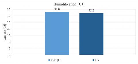
Figure 9. Model validation in terms of humidification
The gas request takes into account both heating and reheating contributions, which are given in Figure 8, and the humidification energy, which is shown in Figure 9. The agreement is very good also for each single contribution.
4.2 Sensitivity analysis to different operating conditions
In order to study the energy performance under different operating conditions, several dynamic simulations have been carried out.
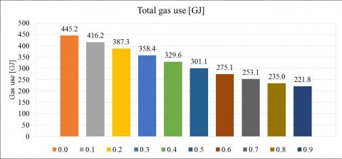
At first, different bps values have been used. The results are shown in Figure 10 and Figure 11 in terms of gas request and cooling energy, respectively. From Figure 10, it is noticeable that the maximum gas request occurs when the entire air flow rate is conditioned in the cooling coil, which corresponds to bps equal to zero. By increasing the fraction of by-passed air flow rate, the gas request decreases, reaching its minimum value at the highest bps coefficient, as expected.
Figure 10. Sensitivity analysis to bps values in terms of total gas request
Figure 11. Sensitivity analysis to bps values in terms of cooling energy
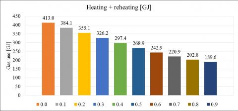
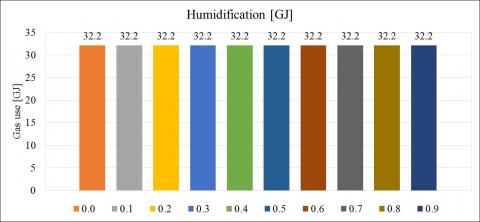
The energy consumption due to cooling and dehumidification processes follows the same trend (Figure 11). Figure 12 and Figure 13 show the contributions of the gas consumption, i.e. the heating+reheating and the humidification energy consumption, respectively. From the figures, it follows that the total gas request consists of a variable contribution (Figure 12) due to sensitive conditioning and a constant contribution (Figure 13) due to the increase of vapor within the mixture given by the humidification process. This contribution does not depend on bps, since it is decoupled from the cooling coil.
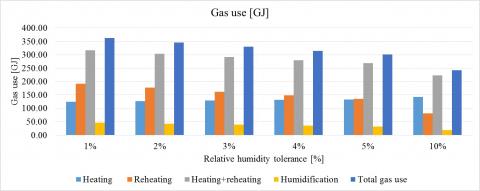
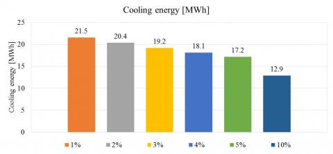
A second analysis deals with the assessment of energy consumption by increasing the acceptable tolerance between the computed relative humidity and the set-point value. The simulations have been carried out by keeping 50 % as comfort humidity and by increasing the tolerance from 1 to 10 %. The results are shown in Figure 14 in terms of gas request and in Figure 15 as regards cooling energy request. It can be noted that by increasing the acceptable tolerance, the gas consumption decreases as a result of the decrease of the energy contributions in terms of reheating and humidification, also if an opposite trend is obtained in terms of heating contribution. This means that lower tolerances involve higher energy consumptions to guarantee the attainment of indoor comfort, as expected. The cooling energy request follows the same trend of the total gas request, as shown in Figure 15.
Figure 12. Sensitivity analysis to bps values in terms of heating and reheating
Figure 13. Sensitivity analysis to bps values in terms of humidification
Figure 14. Sensitivity analysis to relative humidity tolerance in terms of total gas request
Figure 15. Sensitivity analysis to relative humidity tolerance in terms of cooling energy
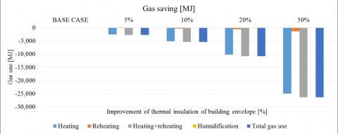
The influence of the thermal insulation of the building envelope has also been investigated. To that end, a gradual increase of the thermal insulation has been considered and different simulations have been carried out. The energy saving has been evaluated by considering an increase of thermal insulation of 5%, 10%, 20% and 50% and the results have been compared with those of the baseline case. As expected, a reduction of thermal transmittance gives a significant decrease of gas request, as shown in Figure 16.
Figure 16. Gas saving by increasing the thermal insulation
With an increase of the thermal insulation of the building envelope, an energy saving of the heating contribution, ranging from 1.5 % to 18.8 % is obtained, with minor changes of the reheating contribution. This is because the reheating energy is due to the heating of moist air after the dehumidification process, which is only slightly affected by the thermal transmittance of the room envelope. Finally, the humidification contribution does not depend at all on the thermal insulation of the building. Table 2 summarizes the results by comparing the data with different thermal insulation.
Table 2. Gas request by increasing the thermal insulation [GJ]
|
BASE CASE |
5% |
10% |
20% |
50% |
|
|
Heating |
133 |
131 |
128 |
123 |
108 |
|
Reheating |
136 |
135 |
135 |
135 |
134 |
|
Humidification |
32 |
32 |
32 |
32 |
32 |
|
Total gas use |
301 |
298 |
296 |
290 |
275 |
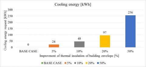
The increase of the building thermal insulation reduces the envelope heat transfer. Therefore, a higher cooling energy requirement is expected in the whole year. As shown in Figure 17, by increasing the thermal transmittance, an additional cooling energy is required up to 256 kWh by increasing the thermal insulation up to 50%.
Figure 17. Additional cooling energy request by increasing thermal insulation
Table 3 summarizes the results of the total cooling energy request. It can be noted that the total cooling energy request increases up to 1.5% by considering an increase of thermal transmittance of 50%.
Table 3. Cooling energy request by increasing the thermal insulation [MWh]
|
BASE CASE |
5% |
10% |
20% |
50% |
|
|
Cooling |
17,160 |
17,184 |
17,208 |
17,257 |
17,416 |
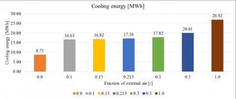
Finally, different fractions of the external air with respect to the recirculation air have been considered. In the baseline case, a fraction equal to 0.787 is assumed, as given in Eq. (2). In what follows, different values of this fraction have been chosen. Specifically, the entire range from 0 to 1 is considered. By assuming this fraction equal to 1, the whole conditioned air comes from the outside and there is no recirculation air. On the other hand, by adopting a value equal to 0 a total recirculation air occurs and it is re-conditioned at each hour. The results are given in Figure 18. The figure shows that by increasing/decreasing the external air flow rate to be conditioned, the gas request increases/decreases.
Figure 18. Gas request with different fractions of external air
The analysis has been performed also in terms of cooling energy request and the results are shown in Figure 19. Like the gas request, the cooling energy consumption increases by increasing the fraction of the external air flow rate.
Figure 19. Cooling energy request with different fractions of external air
Table 4 summarizes the results of the simulations both in terms of gas and cooling energy consumptions. Concerning the consumption of gas, the analysis shows that by assuming that the entire air flow rate to be conditioned comes from the external environment, this energy contribution is about 16 times the consumption obtained by adopting a total air recirculation. Besides the same trend occurs by considering the cooling; in this case the consumption ranges from 9 MWh to 27 MWh.
Table 4. Energy requirement with different fractions of external air
|
0.0 |
0.1 |
0.15 |
0.213 |
0.3 |
0.5 |
1.0 |
|
|
Heating + Reheating |
56 |
212 |
236 |
269 |
317 |
435 |
753 |
|
Humidification |
0 |
15 |
23 |
32 |
45 |
75 |
151 |
|
Total gas use |
57 |
227 |
259 |
301 |
362 |
511 |
904 |
|
Cooling |
9 |
17 |
17 |
17 |
18 |
20 |
27 |
The present work deals with the analysis of advanced conditioning systems and the development of dynamic models that are able to evaluate the energy performance of controlled microclimate. Usually, a significant amount of energy is required to keep optimal microclimate conditions within controlled environments. Besides, strict indoor air quality requirements are often needed both in industrial and residential buildings, thus increasing the energy demand. The aim of this work is to provide a new predictive mathematical model that is an efficient tool to analyze the thermodynamics of conditioning process within controlled environments. The model has been validated with results given in the literature and has been implemented for several control strategies. An iterative algorithm has been implemented to estimate the vapor content in the mixture at the outlet of the conditioned room.
At first, the model validation has been carried out by comparing the results obtained with those given in [1]. Specifically, the comparison has been carried out by adopting an all-air HVAC system with constant air volume for single zone. The analysis is performed by adopting a seasonal set point with indoor air temperature ranging gradually from 21±1 °C to 23±1 °C. The comparison has been performed by considering the annual gas request as regards heating, humidification and reheat processes, whereas dehumidification and cooling contributions have been compared in terms of annual electrical energy request.
In order to improve the efficiency of HVAC, different strategies have been analyzed.
A strategy based on a partial by-pass (bps) of cooling coil is considered to improve the performance of the whole system by guaranteeing the comfort conditions at the same time. The sensitivity analysis to different by-pass amounts shows that the maximum gas request occurs by considering a minimum bps value, conversely the highest performance is obtained with the highest bps, as expected. The same trend occurs also as regards the cooling energy request.
Then, different values of humidity tolerance have been employed and energy consumptions have been evaluated. This analysis provides information about the sensitivity of the model to different ranges of humidity. In this case, by increasing the humidity tolerance, both gas and electrical energy request decrease, as expected.
The effect of the building thermal insulation has also been investigated. The analysis shows that a significant amount of gas request can be avoided by employing different energy requalification strategies able to gain a relevant energy saving. Conversely, an improvement of envelope thermal features involves a very small increase of cooling energy due to the reduction of the heat transfer. In fact, the numerical simulation shows that by considering a very high increase of the thermal insulation, i.e. 50 %, the cooling contribution increases only of about 1.5%.
Finally, different amounts of air recirculation in the microclimate is considered in order to reduce the gas and energy consumptions but preserving the thermal hygrometric comfort conditions. The results show that by reducing the air recirculation the gas request for the conditioning process increases as well as the cooling energy consumption.
|
bps |
fraction of not conditioned air flow rate |
|||
|
G RH |
air flow rate, kg h-1 relative humidity |
|||
|
T |
temperature, °C |
|||
|
Subscripts
|
|
|
||
|
a ext |
air external |
|
||
|
in |
inlet of microclimate environment |
|
||
|
in,cta |
inlet of conditioning unit |
|
||
|
out,cta |
outlet of cooling unit |
|
||
|
rec |
recirculation |
|
||
[1] Ascione F, Bellia L, Capozzoli A, Minichiello F. (2009). Energy saving strategies in air-conditioning for museums. Applied Thermal Engineering 29(4): 676-686. https://doi.org/10.1016/j.applthermaleng.2008.03.040
[2] Camuffo D, Grieken RV, Busse HJ, Sturaro G, Valentino A, Bernardi A, Blades N, Shooter D, Gysels K, Deutsch F, Wieser M, Kim O, Ulrych U. (1999). Environmental monitoring in four European museums. Atmospheric Environment 35(sup1): S127-S140. http://dx.doi.org/10.1016/S1352-2310(01)00088-7
[3] Corgnati SP, Fabi V, Filippi M. (2009). A methodology for microclimatic quality evaluation in museums: Application to a temporary exhibit. Building and Environment 44(6): 1253-1260. http://dx.doi.org/10.1016/j.buildenv.2008.09.012
[4] Pavlogeorgatos G. (2003). Environmental parameters in museums. Building and Environment 38(3): 1457-1462. https://doi.org/10.1016/S0360-1323(03)00113-6
[5] Gysels K, Delalieux F, Deutsch F, Grieken RV, Camuffo D, Bernardi A, Sturaro G, Busse HJ, Wieser M. (2004). Indoor environment and conservation in the Royal Museum of Fine Arts, Antwerp, Belgium. Journal of Cultural Heritage 5(2): 221-230. http://dx.doi.org/10.1016/j.culher.2004.02.002
[6] Camuffo D, Bernardi A, Sturaro G, Valentino A. (2002). The microclimate inside the Pollaiolo and Botticelli rooms in the Uffizi Gallery, Florence. Journal of Cultural Heritage 3(2): 155-161. http://dx.doi.org/10.1016/S1296-2074(02)01171-8
[7] Camuffo D, Brimblecombe P, Grieken RV, Busse HJ, Sturaro G, Valentino A, Bernardi A, Blades N, Shooter D, De Bock L, Gysels K, Wieser M, Kim O. (1999). Indoor air quality at the Correr Museum, Venice, Italy. Science of The Total Environment 236(1-3): 135-152. http://dx.doi.org/10.1016/S0048-9697(99)00262-4
[8] Bellia L, Capozzoli A, Mazzei P, Minichiello F. (2007). A comparison of HVAC systems for artwork conservation. International Journal of Refrigeration 8(8): 1439-1451. http://dx.doi.org/10.1016/j.ijrefrig.2007.03.005
[9] Genco A, Viggiano A, Viscido L, Sellitto G, Magi V. (2016) Numerical simulation of energy systems to control environment microclimate. International Journal of Heat and Technology 34(Special Issue no. 2): S545-S552. http://dx.doi.org/10.18280/ijht.34Sp0249
[10] Genco A, Viggiano A, Viscido L, Sellitto G, Magi V. (2017). Optimization of microclimate control systems for air-conditioned environments. International Journal of Heat and Technology 35(Special Issue no. 1): S236-S243. http://dx.doi.org/10.18280/ijht.35Sp0133
[11] Genco A, Viggiano A, Viscido L, Sellitto G, Magi V. Dynamic analysis of HVAC systems for industrial plants with different airflow control systems. Thermal Science and Engineering Progress, to be published. https://doi.org/10.1016/j.tsep.2017.12.004
[12] Ascione F, Minichiello F. (2010). Microclimatic control in the museum environment: Air diffusion performance. International Journal of Refrigeration 33(4): 806-814. http://dx.doi.org/10.1016/j.ijrefrig.2009.12.017
[13] Zhang XJ, Yu CY, Li S, Zheng YM, Xiao F. (2011). A museum storeroom air-conditioning system employing the temperature and humidity independent control device in the cooling coil. Applied Thermal Engineering 31(17-18): 3653-3657. http://dx.doi.org/10.1016/j.applthermaleng.2010.12.031
[14] Van Schijndel AWM, Schellen HL, Wijffelaars JL, Van Zundert K. (2007). Application of an integrated indoor climate, HVAC and showcase model for the indoor climate performance of a museum. Energy and Buildings 40(4): 647-653. http://dx.doi.org/10.1016/j.enbuild.2007.04.021
[15] https://energyplus.net/weather/sources