OPEN ACCESS
This paper presents a simple correlation and a calculation code for the dynamic simulation of a solar system feeding a radiant floor of a building, able to evaluate the performance of all the components that make up the plant.
Given the qualitative similarities between the thermal field of radiant panels and that of flat solar collectors, in order to obtain a simple and completely analytical expression of the thermal power delivered by the radiant panel to the room to be heated, a calculation methodology similar to that used in the stationary thermal analysis of solar collectors to deduce the Hotel-Whillier-Bliss equation was applied. This methodology has been implemented in a calculation code that resolves discretized thermal balance equations in time domain by applying the finite differences technique. Subsequently, this methodology was implemented in a calculation code.
In order to verify the correctness of the results provided by the simplified correlation and by the calculation code, the solar thermal plant installed at the Department of Mechanical, Energy and Management Engineering (DIMEG) of the University of Calabria was simulated and the results obtained were compared with the experimental data collected with appropriate data acquisition system.
simple correlation, dynamic simulation, solar plant, radiant floor
In recent years, the use of radiant floors as heating and cooling plant for buildings is becoming increasingly widespread [1]. Radiant floors ensure better temperature distribution in the heated space and energy savings compared to traditional heating systems [2]. The possibility of using hot water at low temperature has in itself a twofold advantage [3]: reducing dispersion in the supply circuits and using solar plants which, especially in the winter season, are not able to guarantee, with sufficient autonomy, high temperature levels in the storage tanks [4].
The design phase is fundamental for their use, which must take into account the transient dynamics that are triggered, especially in these types of plants, due to the variability of climatic parameters. For radiant floors, surface temperature estimation and transferred heat are characteristic parameters of fundamental importance [5-6].
The code developed by authors, thanks to the simplicity of the graphical interface, allows to simulate a wide variety of stratigraphies of radiant floors and to change any plant parameter estimating immediately the weight of the parameters on the results obtained.
The most important output of the code is certainly the trend over time of the temperature of storage tank and delivery tank, the average daily temperature and the monthly or hourly average temperature for all the months of the year. In the light of the achievable results, it is possible to make the choices of verification or design that allow constructive optimization and optimal economic management of the plant under examination. The code makes it possible to obtain data for the monthly and annual solar fraction.
Radiant floor plants use low temperature hot water as heat transfer fluid. The heat transfer fluid flows into a drowned serpentine in a concrete screed and provides the necessary heat according to the energy requirements of the room while maintaining an appropriate surface temperature. In reference [7] and in the publication of ASHRAE Handbook, Heating, Ventilating, and Air-Conditioning Systems and Equipment, the main advantages for such type of plants are presented [8].
Since, in a completely experimental way, there were qualitative similarities between the heat field in radiant panels and that existing in flat solar collectors, a calculation methodology similar to that used in the stationary thermal analysis of solar collectors for deducting the Hotel-Whillier-Bliss equation was applied to the radiant panels [9-10]. In this way, a simple, completely analytical expression of the thermal power delivered by the panel to the room to be heated (or subtracted from the environment in case of use of the panel for summer cooling) has been deduced [11]. By means of this equation it is possible to evaluate the thermal yield of the radiant panel and carry out its sizing avoiding any iterative calculation.
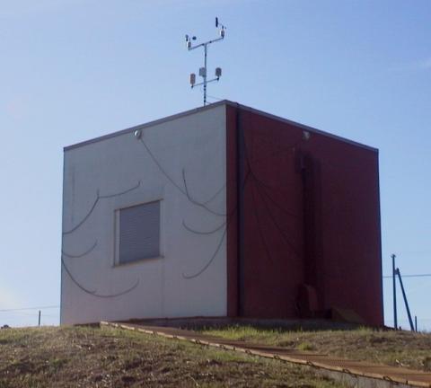
At the Department of Mechanical, Energetics and Management Engineering of the University of Calabria (Italy) a 4x4x3.2 m testing station with variable orientation is functioning, constructed for the study of the thermal behaviour of buildings both with winter heating and with summer air-conditioning, stands on a rotating steel platform (Figure 1).
The thermohygrometric design conditions inside the testing station are guaranteed by a radiant floor, a radiator, a fancoil and of one full air conditioning plant.
The presence of a climate data logger outside the testing station and of numerous PT100 temperature sensors inside the heated space for the acquisition and evaluation of the inside air temperature stratification, and the measurement of the relative humidity complete the data necessary for the evaluation of thermal comfort inside the room.
Figure 1. View of testing station
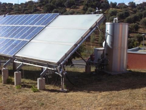
Figure 2 shows an overview of the solar plant that supplies the heat transfer fluid to the radiant floor of testing station, while Figure 3 shows a schematic representation of the system.
The plant shown in Figure 3 consists of a field of solar thermal collectors connected, by means of a heat exchanger, to the storage tank S1, of the supply tank S2 to which a boiler with integration function is connected, of the testing station radiant floor and of the pumps. In addition, the electronic control units equipped with two differential thermostats DT1 and DT2 are installed, capable of putting into operation the solar circuit pump and the pump of the connection circuit of the two tanks.
Figure 2. Thermal solar plant
Figure 3. Schematic representation of the plant
The field of solar collectors collect solar energy and, if the DT1 indicates a temperature difference between the outlet fluid of the collectors and the storage tank, the controller starts up the pump 1 in order to transfer energy into the storage tank. The pump 2 is actuated by the differential thermostats DT2, which, if it reports a temperature difference between the storage tank and the delivery tank, the controller starts up the pump 2 in order transfer energy from the storage tank to the delivery tank by means of the heat transfer fluid.
The flow rate in the radiant floor coil is taken from the delivery tank; the latter is always kept at a minimum temperature thanks to the integration boiler. This boiler, whose fuel is methane, transfers heat to delivery tank if the temperature of that tank falls below the minimum set point value, TS2,min. The system composed by the delivery tank and the radiant floor can be seen as a closed system with constant flow rate. In addition, in the plant is installed a three-way valve, whose function is to guarantee an almost constant temperature of the inlet flow rate to the radiant floor.
The solar system consists of three solar flat collectors with a net capture area of 6 m2. The characteristic curve of the solar collectors is represented by Equation:
$\eta =0.866-4.55\cdot \left( \frac{{{{\bar{T}}}_{f}}-{{T}_{a}}}{{{G}_{c}}} \right)$ (1)
where ${{\bar{T}}_{f}}$ is the average temperature between the inlet temperature, Tin, and the outlet temperature, Tout, of the fluid, Ta is the external air temperature and Gc the global irradiance incident on the collectors plane.
The storage tank used has a capacity of 750 liters. It is teflonized inside, equipped with a finned copper heat exchanger, with a heat transfer surface of 3 m2, mounted on extractable flange. The tank is designed to guarantee a 4-day operating autonomy and is insulated with 10 cm of polyurethane.
The delivery tank is supplied by the storage tank, has a capacity of 100 litres and is not equipped with heat exchanger. The water flow rate sent to the radiant floor is approximately 300 litres/hour at a temperature between 30 °C and 45 °C. When the temperature in the delivery tank drops below 40 °C, the auxiliary boiler starts operating.
The function of the three-way valve (or mixing valve) is to mix the flow rate of hot water coming from the delivery tank with the return flow rate from the radiant floor in order to maintain constant fluid temperature at the inlet of the radiant floor. The mixing valve operates when the flow temperature from the delivery tank is higher than the return flow temperature from the radiant floor.
To avoid overpressure, two expansion vessels, (EV), have been installed in the plant, one on the storage tank and the other on the primary circuit of the collectors.
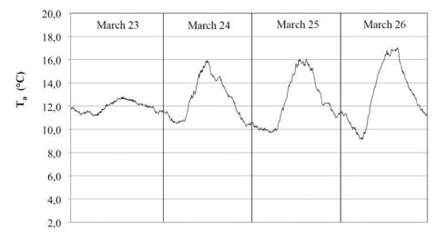
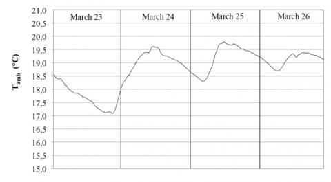
Figure 4, Figure 5 and Figure 6 show, respectively, the trend of solar irradiance detected by the pyranometer on the collectors plane, the external air temperature trend and the temperature trend of the room equipped with radiant floor, related to the period from 23 to 26 March 2016.
Figure 4. Global irradiance incident on the collectors plane from 23 to 26 March 2016
Figure 5. External air temperature from 23 to 26 March 2016
Figure 6. Temperature of the room with radiant floor from 23 to 26 March 2016
The energy conservation equation, referred to, is the one that expresses the first principle of thermodynamics for open systems, non considering, in the case analyzed, contributions related to the work done or absorbed and the variation of the potential and kinetic energy of the system, written for the different components of the considering plant, becomes:
- Solar collectors
${{\dot{m}}_{p}}\,{{c}_{p}}\,\left( {{T}_{out}}-{{T}_{in}} \right)={{F}_{sc}}\,{{F}_{R}}\,{{A}_{c}}\,\left[ {{G}_{c}}\left( \tau \alpha \right)-{{U}_{c}}\left( T{{'}_{S1}}-{{T}_{a}} \right) \right]$ (2)
where $\dot{\mathrm{m}}_{\mathrm{p}}$ is solar collectors mass flow rate, Tout the temperature of outlet flow rate and Tin the temperature of inlet mass flow rate to solar collectors, Fsc the De Winter factor, FR is the radiant floor heat removal factor, Ac is the surface of solar collectors, Gc the global irradiance incident on the collectors plane, (τα) the effective product between the cover transmission coefficient and the plate absorption coefficient, Uc the global heat exchange coefficient of solar collectors, T´S1 the temperature of the fluid in the storage tank in the next time step and Ta the temperature of external air.
- Storage tank:
$\begin{align} & \frac{\rho \,{{V}_{S1}}\,{{c}_{p}}}{\Delta t}\left( T{{'}_{S1}}-{{T}_{S1}} \right)+{{{\dot{m}}}_{s}}\,{{c}_{p}}\,\left( T{{'}_{S1}}-{{T}_{S2}} \right)+{{U}_{S1}}\,{{A}_{S1}}\left( T{{'}_{S1}}-{{T}_{a}} \right)= \\ & ={{F}_{sc}}\,{{F}_{r}}\,{{A}_{c}}\,\left[ {{G}_{c}}\left( \tau \alpha \right)-{{U}_{c}}\left( T{{'}_{S1}}-{{T}_{a}} \right) \right] \\ \end{align}$ (3)
where $\dot{\mathrm{m}}_{\mathrm{s}}$ is the mass flow rate spilled from the storage tank, VS1 the volume of storage tank, TS1 the temperature of the fluid in the storage tank, TS2 the temperature of the fluid in the delivery tank, T´S2 the temperature of the fluid in the delivery tank in the next time step, US1 the global heat exchange coefficient of storage tank and AS1 the storage tank surface.
- Delivery tank:
$\begin{align} & \frac{\rho \,{{V}_{S2}}\,{{c}_{p}}}{\Delta t}\left( T{{'}_{S2}}-{{T}_{S2}} \right)+\left( {{{\dot{m}}}_{u}}-\,{{{\dot{m}}}_{r}} \right)\,{{c}_{p}}\,\left( T{{'}_{S2}}-{{T}_{rfo}} \right)+ \\ & +{{U}_{S2}}\,{{A}_{S2}}\left( T{{'}_{S2}}-{{T}_{a}} \right)={{P}_{in}}\,+{{{\dot{m}}}_{s}}\,{{c}_{p}}\,\left( {{T}_{S1}}-T{{'}_{S2}} \right) \\ \end{align}$ (4)
where $\dot{\mathrm{m}}_{\mathrm{u}}$ is the mass flow rate sent to the radiant floor, ${{\text{\dot{m}}}_{\text{r}}}$the recirculation mass flow rate, VS2 the volume of delivery tank, Trfo the temperature of return flow from the radiant floor, US2 the global heat exchange coefficient of delivery tank, AS2 the delivery tank surface and Pin the power transferred from the boiler to the delivery tank.
- Mixer valve (or three-way valve):
$\dot{m}_{S2}^{{}}\cdot {{h}_{S2}}+\dot{m}_{r}^{{}}\cdot {{h}_{rfo}}={{\dot{m}}_{u}}\cdot {{h}_{rfi}}$ (5)
where $\dot{\mathrm{m}}_{\mathrm{S} 2}$ is the mass flow rate spilled from the delivery tank, hS2 the enthalpy of the inlet mass flow rate to the mixing valve, hrfo the enthalpy of return flow from the radiant floor and hrfi the enthalpy of the inlet flow rate to radiant floor; it has been assumed that ${{h}_{i}}\cong {{c}_{p}}\cdot {{T}_{i}}$.
${{\dot{m}}_{S2}}\cdot {{T}_{S2}}+{{\dot{m}}_{r}}\cdot T_{rfo}^{{}}={{\dot{m}}_{u}}\cdot {{T}_{rfi}}$ (6)
where Trfi is the temperature of the inlet flow to radiant floor; from the Equations (5) and (6) it is possible to obtain the flows to the mixer valve as a function of the known mass flow rate ${{\dot{m}}_{u}}$.
$\left\{ \begin{align} & {{{\dot{m}}}_{S2}}=\left( \frac{{{T}_{rfi}}-{{T}_{rfo}}}{{{T}_{S2}}-{{T}_{rfo}}} \right)\cdot {{{\dot{m}}}_{u}} \\ & \\ & {{{\dot{m}}}_{S2}}+{{{\dot{m}}}_{r}}={{{\dot{m}}}_{u}} \\ \end{align} \right\}$ (7)
Room and its radiant floor:
$\frac{\rho \cdot \,{{c}_{pa}}\,\cdot {{V}_{amb}}\,\left( T{{'}_{amb}}-{{T}_{amb}} \right)}{\Delta t}=({{H}_{T}}+{{H}_{V}})\cdot \,({{T}_{amb}}-{{T}_{a}})$ (8)
where Vamb is the volume of the room, ${{H}_{T}}$ the transmission heat loss coefficient and ${{H}_{V}}$ the design ventilation heat loss coefficient from heated space [12].
The balance equation for the heat exchanger of the storage tank is as follows:
${{\dot{m}}_{p}}\cdot {{c}_{p}}\cdot ({{T}_{out}}-{{T}_{in}})=\varepsilon \cdot {{\dot{m}}_{p}}\cdot {{c}_{p}}\cdot (T_{out}^{{}}-T{{'}_{S1}})$ (9)
where Tout is the outlet temperature of the fluid from solar collectors, Tin the inlet temperature of the fluid from solar collectors, ε represents heat exchanger efficiency.
Combining Equation (2) with Equation (9), the fluid inlet and outlet temperatures from the solar collector are obtained:
$\left\{ \begin{align} & {{T}_{out}}=\frac{{{T}_{in}}}{1-\varepsilon }-\frac{\varepsilon }{1-\varepsilon }T{{'}_{S1}} \\ & {{{\dot{m}}}_{p}}\,{{c}_{p}}\,\left( {{T}_{out}}-{{T}_{in}} \right)={{F}_{sc}}\,{{F}_{r}}\,{{A}_{c}}\,\left[ {{G}_{c}}\left( \tau \alpha \right)-{{U}_{c}}\left( T{{'}_{S1}}-{{T}_{a}} \right) \right] \\ \end{align} \right.$ (10)
In previous equations cp is the specific heat of water and cpa the specific heat of air.
The useful power delivered by the radiant floor to the test space provided by the simplified correlation is as follows:
${{q}_{u}}={{F}_{R}}\cdot {{A}_{p}}\cdot {{U}_{a}}\cdot ({{T}_{rfi}}-{{T}_{amb}})$ (11)
where Ap is the radiant floor surface, Ua the heat transfer coefficient between the upper surface of the concrete layer containing the pipes and the room air, Trfi the inlet temperature to the radiant floor, Tamb the room air temperature and FR is the radiant floor heat removal factor.
The radiant floor heat removal factor can be calculated with the following relation:
${{F}_{R}}=\frac{{{{\dot{m}}}_{u}}\cdot {{c}_{p}}\cdot ({{T}_{rfo}}-{{T}_{rfi}})}{p\cdot L\cdot [{{U}_{a}}({{T}_{rf}}_{i}-{{T}_{amb}})+{{U}_{b}}({{T}_{rf}}_{i}-{{T}_{b}})]}$ (12)
where p is the pitch between pipes, L the length of radiant floor coil, Trfo the outlet temperature from the radiant floor, Ua the global heat exchange coefficient between the radiant panel and the testing space, Ub the global heat exchange coefficient between the radiant panel and the environment below the radiant floor, Tb the temperature of the environment underneath the radiant floor.
The thermal balance equations, previously described, are modified according to the operating conditions of the plant shown in Table 1.
Table 1. Plant operating conditions
|
ΔTDT1 < ΔTdef-DT1 and ΔTDT2 < ΔTdef-DT2 |
No mass flow rate, either from the storage tank or from the delivery tank and the two pumps are not in operation. |
|
ΔTDT1 > ΔTdef-DT1 and ΔTDT2 < ΔTdef-DT2 |
Pump 1 only operates |
|
ΔTDT1 < ΔTdef-DT1 and ΔTDT2 > ΔTdef-DT2 |
Pump 2 only operates |
|
ΔTDT2 > ΔTdef-DT2 and operating mode on |
Pin = 0 and the plant sends a constant mass flow rate to the radiant floor |
|
ΔTDT2 > ΔTdef-DT2 and operating mode off |
Pin = 0 and the plant does not send a constant mass flow rate to the radiant floor, ${{\dot{m}}_{u}}-{{\dot{m}}_{r}}=0$ |
|
ΔTDT2 < ΔTdef-DT2 and operating mode on and TS2 >T S2,min |
Pin = 0 and ${{\dot{m}}_{s}}=0$ |
|
ΔTDT2 < ΔTdef-DT2 and operating mode off and TS2 >T S2,min |
Pin =0, ${{\dot{m}}_{s}}=0$ and ${{\dot{m}}_{u}}-{{\dot{m}}_{r}}=0$ |
|
ΔTDT2 < ΔTdef-DT2 and operating mode on and TS2 < T S2,min |
Pin $\ne $ 0 and ${{\dot{m}}_{s}}=0$ |
|
ΔTDT2 <ΔTdef-DT2 and operating mode off and TS2 < T S2,min |
Pin $\ne $ 0, ${{\dot{m}}_{s}}=0$ and ${{\dot{m}}_{u}}-{{\dot{m}}_{r}}=0$ |
|
TS2 < Trfi |
${{\dot{m}}_{s2}}={{\dot{m}}_{u}}$ |
|
Tamb > Tsetpoint |
${{\dot{m}}_{u}}={{\dot{m}}_{r}}$ and ${{\dot{m}}_{S2}}=0$ |
|
Tamb < Tsetpoint |
${{\dot{m}}_{u}}={{\dot{m}}_{S2}}$ and ${{\dot{m}}_{r}}=0$ |
The equations and the operating conditions of the plant, described above, have been implemented in a computer code. The code allows to estimate the trend of the hourly and monthly average temperature of the water in the two tanks, the amount of energy provided by the primary circuit, the amount of energy transferred to the environment where the radiant floor is placed and the amount of integration energy. In addition, the use of the code allows a quick calculation of the only radiant floor not connected to the solar plant. The calculation code allows estimate any parameter related to the radiant floor requiring as input data only the temperature of the fluid inlet to the floor itself.
Furthermore allows to choose the location where the plant will be located, the type of radiant floor to be simulated, to enter all plant parameters, the mass flow rate of the inlet fluid to the radiant floor at different hours of the day, the default difference temperature of the differential thermostats, the characteristics of the coil to assess the heat exchanger efficiency in the storage tank, the radiant floor stratigraphy, the parameters characterizing the environment in which the radiant floor is located and the mixer valve operation mode.
The experimental data recorded at the test station every 5 minutes for the period from 23 March to 23 April 2016 have been used for the validation of the code. The radiant floor has been kept in operation continuously in order to establish almost stationary conditions inside the room. When the set-point temperature for the heating space (Tsetpoint = 20 °C) is reached, the room thermostat acting on the three-way valve sends the entire bypass flow rate to the radiant floor. A similar operation is carried out by means of the maximum temperature probe if the temperature of the flow rate of water entering the radiant floor exceeds a set value of 45 °C. The mass flow rate of the coil was maintained constant and equal to 300 l/h, while the input flow rate temperature varied between 30 °C and 45 °C.
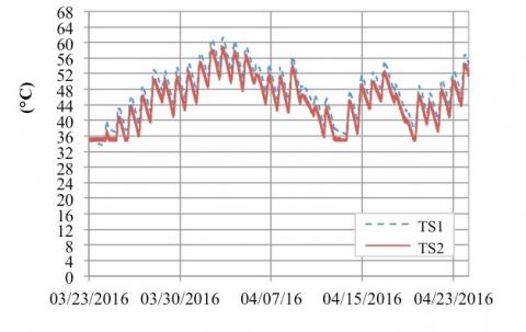
Figure 7 shows the experimental indoor and outdoor air temperature throughout the test period considered. Figure 8 shows the trend of solar radiation measured by the pyranometer located on the collectors plane, inclined of 39° respect to the horizontal plane. Figure 9 shows the experimental temperatures of the water in the two tanks.
Figure 7. Experimental indoor and outdoor air temperature for the period from March 23 to April 23, 2016
Figure 8. Solar radiation on collectors plane for the period from March 23 to April 23, 2016
Figure 9. Experimental water temperature in the two tanks for the period from March 23 to April 23, 2016
Table 2 shows the technical parameters of the simulated solar plant, while Table 3 shows the technical characteristics of the storage tank heat exchanger. The parameters are those relating to the system installed at the test station located in Arcavacata di Rende (Italy).
Table 4 shows the thickness and thermal conductivity of the materials that make up the stratigraphy of the radiant floor. The coil, through which heat is supplied to the environment, is made of copper and is embedded in the concrete.
It is necessary to know the evolution of the fluid temperature in the two tanks depending on their thermal losses, the energy absorbed for heating by the radiant floor, the energy input from the primary circuit and the dynamic interaction between the two tanks.
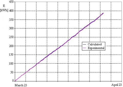
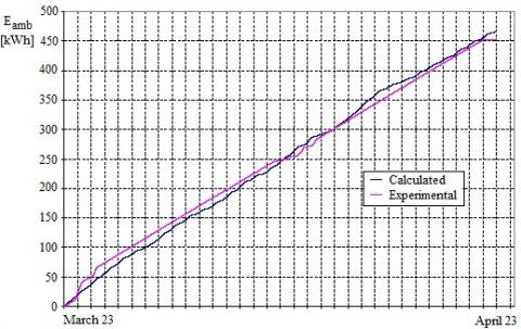
Figure 10 shows the comparison between the experimental cumulated energy provided by the primary circuit (upstream of the storage tank) and that calculated with the simplified model.
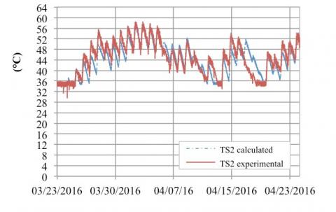
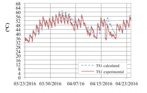
Figure 11 shows the experimental and calculated values of the fluid temperature in the storage tank. The results showed an average deviation of -0.97% and an RMSE (Root Mean Square Error) value of 5.47%. Instead, Figure 12 shows the experimental and calculated values of the fluid temperature in the delivery tank. In this case the results showed an average deviation of -2.49% and a RMSE of 6.76%. Finally, as regards energy transferred to the environment from the radiant floor, the average deviation is equal to 8% and the RMSE equal to 18%.
In Figure 13 a comparison is made between the calculated and experimental power delivered by the primary circuit.
Table 2. Technical parameters of the solar plant
|
Surface of solar collectors [m2] |
6 |
|
Inner diameter of solar collectors pipes [m] |
0.02 |
|
Outer diameter of solar collectors pipes [m] |
0.025 |
|
Length of solar collectors pipes [m] |
12 |
|
Global heat exchange coefficient of solar collectors [W/(m2 K)] |
7.2 |
|
Inclination angle of solar collectors [°] |
39 |
|
Volume of storage tank [m3] |
0.75 |
|
Volume of delivery tank [m3] |
0.1 |
|
Global heat exchange coefficient of storage tank [W/(m2 K)] |
0.47 |
|
Global heat exchange coefficient of delivery tank [W/(m2 K)] |
0.47 |
|
Storage tank surface [m2] |
3.56 |
|
Delivery tank surface [m2] |
1.62 |
|
Length of pipes from the delivery tank [m] |
34 |
|
Mass flow rate of the primary circuit (collector- storage tank) [kg/s] |
0.125 |
|
ΔTdef-DT1 of differential thermostat DT1 [°C] |
3 |
|
ΔTdef-DT2 of differential thermostat DT2 [°C] |
3 |
|
Temperature of inlet flow to radiant floor [°C] |
30 |
Table 3. Technical characteristics of the heat exchanger
|
Outer diameter of the pipe [m] |
0.025 |
|
Inner diameter of the pipe [m] |
0.02 |
|
Serpentine length [m] |
15 |
|
Thermal conductivity of the serpentine [W/(m K)] |
400 |
Table 4. Stratigraphy of the radiant floor
|
Material |
Thermal conductivity [W/(m K)] |
Thickness [m] |
|
Tiles |
1.0 |
0.01 |
|
Concrete |
0.7 |
0.05 |
|
Insulating |
0.035 |
0.3 |
|
Concrete |
0.7 |
0.15 |
Figure 10. Calculated and experimental cumulated energy provided by the primary circuit
Figure 11. Calculated and experimental delivery tank temperature
Figure 12. Calculated and experimental storage tank temperature
Figure 13. Calculated and experimental power delivered from the primary circuit
In Figure 14, the comparison between calculated and experimental cumulated energy transferred to the environment, when the radiant floor plant is functioning, is reported. During the period considered, the solar fraction was 86%, i.e. 14% of the load required by the environment was supplied by the boiler while the remaining 86% by the solar collectors.
Figure 14. Calculated and experimental cumulated energy transferred to the room
In order to have a further verification of the validity of the simplified model and of the code, a simulation on an annual basis of the same plant located in Cosenza and Turin was carried out, utilizing the climatic data furnished by Italian norms. It has been assumed that the plant operates during the heating periods provided for by Italian legislation: 15 November until 31 March for Cosenza and 15 October until 15 April for Turin. For the simulations, the following operating conditions have been fixed: the fluid temperature in the two tanks at the initial instant is equal to 40 °C, the boiler ignition occurs when the temperature of the delivery tank drops below 45 °C and mixer valve adjustment occurs when the environmental temperature drops below 20 °C.
4.1 Results for the plant installed in Cosenza
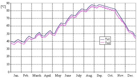
Figures 15 and 16 show, respectively, the trend of fluid temperature in the two tanks and the energy released from the radiant floor in the case of plant installed in Cosenza for the year 2016.
The value of the annual solar fraction obtained is equal to 0.63.
Figure 15. Trend of fluid temperature in the two tanks for the plant installed in Cosenza
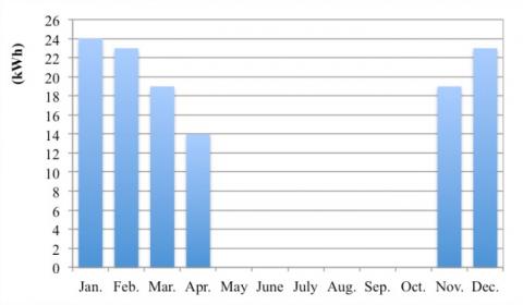
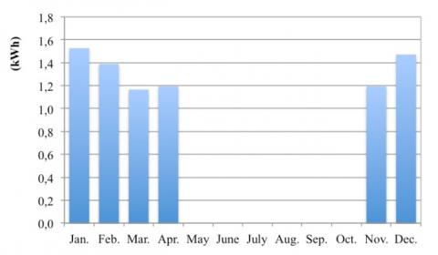
Figure 16. Energy released from the radiant floor for the plant installed in Cosenza
4.2 Results for the plant installed in Turin
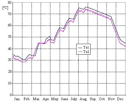
Figures 17 and 18 show, respectively, the trend of fluid temperature in the two tanks and the energy released from the radiant floor in the case of the plant installed in Turin for the year 2016. The value of the annual solar fraction obtained is equal to 0.32.
Figure 17. Trend of fluid temperature in the two tanks for the plant installed in Turin
Figure 18. Energy released from the radiant floor for the plant installed in Turin
In this paper a simple correlation implemented in a calculation code able to perform dynamic simulation and estimate the performance of a solar thermal system connected to a radiant floor is presented.
The code is able to simulate the behaviour of different stratigraphies of radiant floors and evaluate the weight that each component of the solar system can have on the system itself.
The calculation code has been validated by using the experimental data of the solar thermal plant installed at the Department of Mechanical, Energy and Management Engineering (DIMEG) of the University of Calabria, comparing the results obtained by the code with the experimental data collected by suitable measuring instruments.
The simulations performed showed a good agreement between the calculated results and experimental data. As far as energy supplied by the primary circuit is concerned, an average deviation between experimental data and those calculated with the code of 0.8% and an RMSE value of 1.83% has been estimated.
Regarding the fluid temperature in the storage tank, an average deviation of -0.97% between calculated results and experimental data was evaluated and an RMSE value of 5.47%; for the fluid temperature in the delivery tank, an average deviation of -2.49% and an RMSE of 6.76% was evaluated. As regards energy transferred to the environment from the radiant floor, the average deviation is equal to 8% and the RMSE equal to 18%.
Finally, in order to better verify the validity of the code, additional annual simulations have been implemented for two different Italian locations: Cosenza and Turin. These simulations made it possible to evaluate the performance of the solar system when it is located in different locations to assess the influence of the climate.
The analysis also estimated the annual solar fraction of the plant for the two sites, equal to 0.63 for the city of Cosenza and to 0.32 for the city of Turin.
|
Ac |
Surface of solar collectors (m2) |
|||
|
Ap |
Radiant floor surface (m2) |
|||
|
AS1 |
Storage tank surface (m2) |
|||
|
AS2 |
Delivery tank surface (m2) |
|||
|
cpa |
Specific heat of air (J kg-1 K-1) |
|||
|
cp |
Specific heat of the fluid (J kg-1 K-1) |
|||
|
FR |
Radiant floor heat removal factor |
|||
|
DT1 |
Differential thermostat 1 |
|||
|
DT2 |
Differential thermostat 2 |
|||
|
Fsc |
De Winter factor |
|||
|
Gc |
Global irradiance incident on the collectors plane (W m-2) |
|||
|
${{H}_{T}}$ |
Transmission heat loss coefficient from heated space (W K-1) |
|||
|
${{H}_{V}}$ |
Design ventilation heat loss coefficient from heated space (W K-1) |
|||
|
hS2 |
Enthalpy of the inlet flow rate to the mixing valve (J kg-1) |
|||
|
hrfo |
Enthalpy of outlet flow rate from the radiant floor (J kg-1) |
|||
|
hrfi |
Enthalpy of inlet flow rate to radiant floor (J kg-1) |
|||
|
L |
Length of radiant floor coil (m) |
|||
|
$\dot{\mathrm{m}}_{\mathrm{p}}$ |
Solar collector mass flow rate (kg s-1) |
|||
|
$\dot{\mathrm{m}}_{\mathrm{r}}$ |
Recirculation mass flow rate to mixing valve (kg s-1) |
|||
|
$\dot{\mathrm{m}}_{\mathrm{s}}$ |
Mass flow rate spilled from the storage tank (kg s-1) |
|||
|
$\dot{\mathrm{m}}_{\mathrm{S} 2}$ |
Mass flow rate spilled from the delivery tank (kg s-1) |
|||
|
$\dot{\mathrm{m}}_{\mathrm{u}}$ |
Mass flow rate sent to the radiant floor (kg s-1) |
|||
|
p |
Pitch between pipes (m) |
|||
|
Pin |
Power transferred from the boiler to the delivery tank (W) |
|||
|
qu |
Useful power delivered by radiant floor to the test space (W) |
|||
|
Ta |
Temperature of external air (°C) |
|||
|
Tamb |
Temperature of testing space with radiant floor (°C) |
|||
|
T´amb |
Temperature of testing space with radiant floor in the next time step (°C) |
|||
|
Tb |
Temperature of the environment underneath the radiant floor (°C) |
|||
|
Tin |
Temperature of inlet flow to solar collectors (°C) |
|||
|
Tout |
Temperature of outlet flow from solar collectors (°C) |
|||
|
Trfi |
Temperature of inlet flow to radiant floor (°C) |
|||
|
Trfo |
Temperature of return flow from radiant floor (°C) |
|||
|
Tsetpoint |
Set point temperature of testing space with radiant floor (°C) |
|||
|
TS1 |
Temperature of the fluid in the storage tank (°C) |
|||
|
T´S1 |
Temperature of the fluid in the storage tank in the next time step (°C) |
|||
|
TS2 |
Temperature of the fluid in the delivery tank (°C) |
|||
|
T´S2 |
Temperature of the fluid in the delivery tank in the next time step (°C) |
|||
|
Tmin,S2 |
Minimum temperature of the fluid in the delivery tank (°C) |
|||
|
Ua |
Global heat exchange coefficient between the radiant panel and the testing space (W m-2 K-1) |
|||
|
Ub |
Global heat exchange coefficient between the radiant panel and the environment below the radiant floor (W m-2 K-1) |
|||
|
Uc |
Global heat exchange coefficient of solar collectors (W m-2 K-1) |
|||
|
US1 |
Global heat exchange coefficient of storage tank (W m-2 K-1) |
|||
|
US2 |
Global heat exchange coefficient of delivery tank (W m-2 K-1) |
|||
|
Vamb |
Volume of testing space (m3) |
|||
|
VS1 |
Volume of storage tank (m3) |
|||
|
VS2 |
Volume of delivery tank (m3) |
|||
|
Greek symbols
|
|
|
||
|
ΔT |
Temperature difference (°C) |
|
||
|
Δt |
Time path (s) |
|
||
|
ΔTdef-DT1 |
Design temperature difference for differential thermostat DT1 |
|
||
|
ΔTdef-DT2 |
Design temperature difference for differential thermostat DT2 |
|
||
|
ε |
Heat exchanger efficiency |
|
||
|
η |
Solar collectors efficiency |
|
||
|
ρ |
Fluid density (kg m-3) |
|
||
|
(τα) |
Effective product between the cover transmission coefficient and the plate absorption coefficient |
|
||
[1] Márquez AA, López JMC, Hernández FF, Muñoz FD, Andrés AC. (2017). A comparison of heating terminal units: Fan-coil versus radiant floor, and the combination of both. Energy and Buildings 138: 621-629. https://doi.org/10.1016/j.enbuild.2016.12.092
[2] Olesen BW. (2002). Radiant floor heating in theory and practice. ASHRAE Journal 44(7): 19-24.
[3] Bojić M, Cvetković D, Marjanović V, Blagojević M, Djordjević Z. (2013). Performances of low temperature radiant heating systems. Energy and Buildings 61: 233-238. https://doi.org/10.1016/j.enbuild.2013.02.033
[4] Bojić M, Cvetković D, Bojić L. (2015). Decreasing energy use and influence to environment by radiant panel heating using different energy sources. Energy and Buildings 138: 404-413. https://doi.org/10.1016/j.apenergy.2014.10.063
[5] Wu X, Zhao BJ, Olesenc BW, Fangc L, Wang F. (2015). A new simplified model to calculate surface temperature and heat transfer of radiant floor heating and cooling systems. Energy and Buildings 105: 285-293. http://dx.doi.org/10.1016/j.enbuild.2015.07.056
[6] Cholewa T, Rosinskib M, Spikb Z, Dudzinskaa MR, Siuta-Olcha A. (2013). On the heat transfer coefficients between heated/cooled radiant floorand room. Energy and Buildings 66: 599-606. http://dx.doi.org/10.1016/j.enbuild.2013.07.065
[7] Shin MS, Rhee KN, Ryu SR, Yeo MS, Kim KR. (2015). Design of radiant floor heating panel in view of floor surface temperatures. Building and Environment 92: 559-577. http://dx.doi.org/10.1016/j.buildenv.2015.05.006
[8] Atlanta GA. (2012). ASHRAE Handbook, Heating, Ventilating, and Air-Conditioning Systems and Equipment, SI edition, ISSN 1041-2344.
[9] Hottel HC, Whillier A. (1958). evaluation of flat-plate collector performance, transactions of the conference on use of solar energy. University of Arizona Press 2: 74-78. https://doi.org/10.1155/2012/686393.
[10] Bliss RW. (1959). the derivations of several ‘plate efficiency factors’ useful in the design of flat-plate solar-heat collectors. Solar Energy 3(4): 55-64. https://doi.org/10.1016/0038-092X(59)90006-4
[11] Cucumo M, Ferraro V, Kaliakatsos D, Marinelli V. (1999). Radiant floors. A simplified method of calculation and its experimental validation, CDA, Condizionamento dell Aria. Riscaldamento e Refrigerazione 5: 453-461.
[12] EN 12831:2017 - Energy performance of buildings - Method for calculation of the design heat load - Part 1: Space heating load, Module M3-3, ICS: [91.140.10].