OPEN ACCESS
This paper examines synchronization between two identical 6-D hyperchaotic Lorenz systems based on nonlinear control strategy. The designed control functions for the synchronization between the drive state variables and the response state variables are succeed to achieve synchronization with unknown parameters. Numerical simulations are carried out to validate the effectiveness of the analytical technique.
chaos synchronization, 6-D hyperchaotic Lorenz system, nonlinear control strategy, Lyapunov stability theory, linearization method
Chaos control is one of the chaos treatments, which contains two aspects, namely, chaos control and chaos synchronization. Chaos control can be classified into two categories: one is to suppress the chaotic dynamical behavior when it is harmful or is attempt to eliminate chaotic behavior, and the other is to generate or enhance chaos when it is desirable known as chaotification or anti-control of chaos [1].
Synchronization means to control a chaotic system to follow another chaotic system. Chaos control and chaos synchronization were once believed to be impossible until the 1990s when Ott et al. developed the OGY method to suppress chaos [2]. Pecora and Carroll introduced a method to synchronize two identical chaotic systems with different initial conditions [3], which opens the way for chaotic systems synchronization. Chaos control and chaos synchronization play very important role in the study of nonlinear dynamical systems and have great significance in the application of chaos [4]. Especially, the subject of chaos synchronization has received considerable attention due to its potential applications in physics [5], secure communication, chemical reactor, biological networks, control theory, artificial neural network. etc. [6].
Various types of synchronization phenomena have been presented such as complete synchronization (CS), generalized synchronization (GS), lag synchronization, anti-synchronization (AS), projective synchronization (PS), generalized projective synchronization (GPS). The most familiar synchronization phenomena are complete synchronization and anti-synchronized [7, 8].
In the last two decades, extensive studies have been done on the properties of nonlinear dynamical systems. One of the most important properties of nonlinear dynamical systems is that of chaos [9]. This phenomenon is an important topic in nonlinear science and has been intensively investigated within the mathematics, physics, engineering science, and secure communication, etc. [6, 8, 9]. Chaos is sometimes undesirable, so, we wish to avoid and eliminate such behaviors [10]. Therefore, chaos control has become the key process in applying chaos. Since Ott, Grebogi and Yorke (OGY) firstly proposed the method of chaos control in 1990, thereafter enormous research activates have been carried out in chaos control by many researchers from different disciplines, and lots of successful experiments have been reported
Chaotic system has become an important aspect in dynamical systems due to its interesting and complex dynamical behaviors. But, for this system, there is just one positive Lyapunov exponent. In secure communication, messages masked by such simple chaotic systems are not always safe [11]. It is suggested that this problem can be overcome by using higher-dimensional hyperchaotic systems, which have increased randomness and higher unpredictability. Due to its higher unpredictability than chaotic systems, the hyperchaos may be more useful in some fields such as secure communication [12]. So, it's needed to discover hyperchaotic systems, these systems are characterized as a chaotic system with more than one positive Lypunov exponent, and have more complex and richer dynamical behaviors than chaotic system. Historical, Rössler system is the first hyperchaotic systems which discover in 1979, Since then, many hyperchaotic systems have been discover [13], such as hyperchaotic Lorenz system [2], hyperchaotic Liu system, hyperchaotic Chen system, Modified hyperchaotic Pan system (2012), as well as to propose a 5-D hyperchaotic system such as A novel 5-D hyperchaotic Lorenz system (2014), a novel hyperjerk system with two nonlinearities. Currently, a novel 6-D hyperchaotic Lorenz is discover by Yang which contains four positive Lyapunov Exponents [16].
The main contribution of this paper is the achieving synchronzation between two identical 6-D hyperchaotic Lorenz system via nonlinear control strategy with unknown parameters.
In 2015, Yang constructed a 6-D hyperchaotic system which include 14 terms, three of them are nonlinearity i.e., $x _ { 1 } x _ { 3 } , x _ { 1 } x _ { 2 } , x _ { 1 } x _ { 3 }$ for the second, third and fourth equation, respectively[15]. And its contains four positive Lyapunov Exponents $L E _ { 1 } = 1.0034 , L E _ { 2 } = 0.57515 , L E _ { 3 } = 0.32785$, $L E _ { A } = 0.020937$ and two negative Lyapunov Exponents $L E _ { 5 } = - 0.12087 , L E _ { 6 } = - 12.4713$. The dynamics of Lorenz system is given by the following form
$\left\{ \begin{array} { l } { \dot { x } _ { 1 } = a \left( x _ { 2 } - x _ { 1 } \right) + x _ { 4 } } \\ { \dot { x } _ { 2 } = c x _ { 1 } - x _ { 2 } - x _ { 1 } x _ { 3 } + x _ { 5 } } \\ { \dot { x } _ { 3 } = - b x _ { 3 } + x _ { 1 } x _ { 2 } } \\ { \dot { x } _ { 4 } = d x _ { 4 } - x _ { 1 } x _ { 3 } } \\ { \dot { x } _ { 5 } = - k x _ { 2 } } \\ { \dot { x } _ { 6 } = l x _ { 2 } + h x _ { 6 } } \end{array} \right.$ (1)
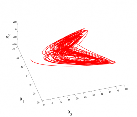
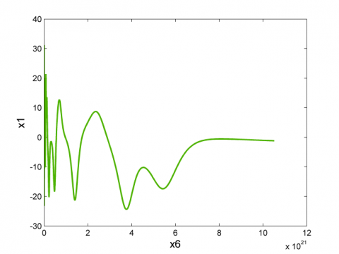
where $a , b , c , d , k , l$ and $h$ are constant and $x _ { i } , i = 1,2 , \dots , 6$ are a state variables. The Lorenz system shows hyperchaotic behaviour when $a = 10 , b = \frac { 8 } { 3 } , c = 28 , d = 2 , k = 8.4 , l = 1$ and $h = 1$. Figures 1-3 show the 3-D attractor of the system (1), while figures 4-6 show the 2-D attractor of the system (1).
Figure 1. 3-D attractor of the system (1) in the $\left( x _ { 1 } , x _ { 3 } , x _ { 4 } \right)$ space
Figure 2. 3-D attractor of the system (1) in the $\left( x _ { 1 } , x _ { 3 } , x _ { 5 } \right)$ space
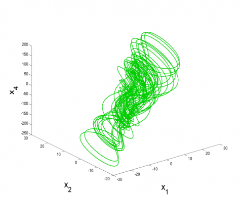
Figure 3. 3-D attractor of the system (1) in the $\left( x _ { 1 } , x _ { 2 } , x _ { 4 } \right)$ space
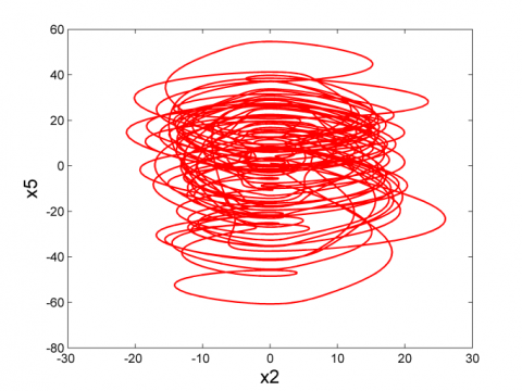
Figure 4. 2-D attractor of the system (1) in the $\left( x _ { 2} , x _ { 5} \right)$ plane
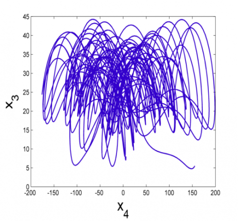
Figure 5. 2-D attractor of the system (1) in the $\left(x _ { 3 } , x _ { 4 } \right)$ plane
Figure 6. 2-D attractor of the system (1) in the $\left( x _ { 1 } , x _ { 6 } \right)$ plane
Our purpose herein is to realize complete synchronization between identical 6-D hyperchaotic Lorenz systems by the nonlinear control technique with unknown parameters. To begin with, the definition of chaos synchronization used in this paper is given as
3.1 Definition
For two nonlinear dynamical systems:
$\dot { X } _ { i } = F _ { 1 } \left( X _ { i } \right)$ (2)
$\dot { Y } _ { i } = F _ { 2 } \left( Y _ { i } \right) + U \left( X _ { i } , Y _ { i } \right)$ (3)
where $X _ { i } , Y _ { i } \in R ^ { n } , F _ { 1 } , F _ { 2 } : R ^ { n } \rightarrow R ^ { n } , i = 1,2 , \ldots , n , U \left( X _ { i } , Y _ { i } \right)$ is the nonlinear control vector, suppose that Eq. (2) is the drive system, Eq. (3) is the response system. The response system and drive system are said to be chaos synchronized or (complete /full) synchronized if for
$\forall X _ { i } , Y _ { i } \in R ^ { n } , \lim _ { t \rightarrow } \infty \left\| Y _ { i } - \alpha _ { i } X _ { i } \right\| = 0$
where $\alpha _ { i }$ is the scaling factor taken the value 1 for complete synchronization.
3.2 Design of nonlinear controllers
According to the above definition, we consider system (1) as the drive system and the response system is given as the following form:
$\left\{ \begin{array} { l } { \dot { y } _ { 1 } = a \left( y _ { 2 } - y _ { 1 } \right) + x _ { 4 } + u _ { 1 } } \\ { \dot { y } _ { 2 } = c y _ { 1 } - y _ { 2 } - y _ { 1 } y _ { 3 } + y _ { 5 } + u _ { 2 } } \\ { \dot { y } _ { 3 } = - b y _ { 3 } + y _ { 1 } y _ { 2 } + u _ { 3 } } \\ { \dot { y } _ { 4 } = d y _ { 4 } - y _ { 1 } y _ { 3 } + u _ { 4 } } \\ { \dot { y } _ { 5 } = - k y _ { 2 } + u _ { 5 } } \\ { \dot { y } _ { 6 } = l y _ { 2 } + h y _ { 6 } + u _ { 6 } } \end{array} \right.$ (4)
where $U = \left[ u _ { 1 } , u _ { 2 } , u _ { 3 } , u _ { 4 } , u _ { 5 } , u _ { 6 } \right] ^ { T }$ is the nonlinear controller to be designed.
The synchronization error $e _ { i } \in R ^ { 6 }$ for CS is defined as
$\left\{ \begin{array} { l } { e _ { 1 } = y _ { 1 } - x _ { 1 } } \\ { e _ { 2 } = y _ { 2 } - x _ { 2 } } \\ { e _ { 3 } = y _ { 3 } - x _ { 3 } } \\ { e _ { 4 } = y _ { 4 } - x _ { 4 } } \\ { e _ { 5 } = y _ { 5 } - x _ { 5 } } \\ { e _ { 6 } = y _ { 6 } - x _ { 6 } } \end{array} \right.$
According to the above system, the error dynamics is calculated as the following:
$\left[ \begin{array} { c } { \dot { e } _ { 1 } } \\ { \dot { e } _ { 2 } } \\ { \dot { e } _ { 3 } } \\ { \dot { e } _ { 4 } } \\ { \dot { e } _ { 5 } } \\ { \dot { e } _ { 6 } } \end{array} \right] = A \left[ \begin{array} { c } { e _ { 1 } } \\ { e _ { 2 } } \\ { e _ { 3 } } \\ { e _ { 4 } } \\ { e _ { 5 } } \\ { e _ { 6 } } \end{array} \right] + \left( B D + \left[ \begin{array} { c } { u _ { 1 } } \\ { u _ { 2 } } \\ { u _ { 3 } } \\ { u _ { 4 } } \\ { u _ { 5 } } \\ { u _ { 6 } } \end{array} \right] \right)$ (5)
where
$A = \left[ \begin{array} { c c c c c c } { - a } & { a } & { 0 } & { 1 } & { 0 } & { 0 } \\ { c } & { - 1 } & { 0 } & { 0 } & { 1 } & { 0 } \\ { 0 } & { 0 } & { - b } & { 0 } & { 0 } & { 0 } \\ { 0 } & { 0 } & { 0 } & { d } & { 0 } & { 0 } \\ { 0 } & { - k } & { 0 } & { 0 } & { 0 } & { 0 } \\ { 0 } & { l } & { 0 } & { 0 } & { 0 } & { h } \end{array} \right]$
$B = \left[ \begin{array} { l l l } { 0 } & { 0 } & { 0 } \\ { 1 } & { 0 } & { 0 } \\ { 0 } & { 1 } & { 0 } \\ { 0 } & { 0 } & { 1 } \\ { 0 } & { 0 } & { 0 } \\ { 0 } & { 0 } & { 0 } \end{array} \right]$
$D = \left[ \begin{array} { c } { - e _ { 1 } e _ { 3 } - x _ { 3 } e _ { 1 } - x _ { 1 } e _ { 3 } } \\ { e _ { 1 } e _ { 2 } + x _ { 2 } e _ { 1 } + x _ { 1 } e _ { 2 } } \\ { - e _ { 1 } e _ { 3 } - x _ { 3 } e _ { 1 } - x _ { 1 } e _ { 3 } } \end{array} \right]$
Then system (5) can be redefined as
$\left\{ \begin{array} { l } { \dot { e } _ { 1 } = a \left( e _ { 2 } - e _ { 1 } \right) + e _ { 4 } + u _ { 1 } } \\ { \dot { e } _ { 2 } = c e _ { 1 } - e _ { 2 } + e _ { 5 } - e _ { 1 } e _ { 3 } - x _ { 3 } e _ { 1 } - x _ { 1 } e _ { 3 } + u _ { 2 } } \\ { \dot { e } _ { 3 } = - b e _ { 3 } + e _ { 1 } e _ { 2 } + x _ { 1 } e _ { 2 } + x _ { 2 } e _ { 1 } + u _ { 3 } } \\ { \dot { e } _ { 4 } = d e _ { 4 } - e _ { 1 } e _ { 3 } - x _ { 3 } e _ { 1 } - x _ { 1 } e _ { 3 } + u _ { 4 } } \\ { \dot { e } _ { 5 } = - k e _ { 2 } + u _ { 5 } } \\ { \dot { e } _ { 6 } = l e _ { 2 } + h e _ { 6 } + u _ { 6 } } \end{array} \right.$ (6)
Based on linearization method we obtain the following
$\left| \begin{array} { c c c c c c } { ( - 10 - \lambda ) } & { 10 } & { 0 } & { 1 } & { 0 } & { 0 } \\ { 28 } & { ( - 1 - \lambda ) } & { 0 } & { 0 } & { 1 } & { 0 } \\ { 0 } & { 0 } & { \left( - \left( \frac { 8 } { 3 } \right) - \lambda \right) } & { 0 } & { 0 } & { 0 } \\ { 0 } & { 0 } & {0} & {( 2-\lambda )} & { 0 } & { 0 } \\ { 0 } & { - 8.4 } & { 0 } & { 0 } & { - \lambda} & { 0 } \\ { 0 } & { 1 } & { 0 } & { 0 } & { 0 } & { ( 1 - \lambda ) } \end{array} \right|=0$
and the characteristic equation has the forms:
$\lambda ^ { 6 } + \frac { 32 } { 3 } \lambda ^ { 5 } - \frac { 4069 } { 15 } \lambda ^ { 4 } + \frac { 1658 } { 15 } \lambda ^ { 3 } + \frac { 24004 } { 15 } \lambda ^ { 2 } - \frac { 9496 } { 5 } \lambda+448=0$
The six roots of the above equation are
$\left\{ \begin{array} { l } { \lambda _ { 1 } = 1 } \\ { \lambda _ { 2 } = 2 } \\ { \lambda _ { 3 } = - \frac { 8 } { 3 } } \\ { \lambda _ { 4 } = 11.36592689 - 8.10 ^ { - 9 } i } \\ { \lambda _ { 5 } = - 22.69162026 - 3.92820323010 ^ { - 9 } i } \\ { \lambda _ { 6 } = 0.32569338 + 9.92820323010 ^ { - 9 } i } \end{array} \right.$
So, some roots with positive real parts. Consequently, we must design control in order to suppresses this error dynamics (6).
Theorem 1. For the error dynamics system (system 6) with nonlinear control $U = \left[ u _ { 1 } , u _ { 2 } , u _ { 3 } , u _ { 4 } , u _ { 5 } , u _ { 6 } \right] ^ { T }$ such that
$\left\{ \begin{array} { l } { u _ { 1 } = x _ { 3 } \left( e _ { 2 } + e _ { 4 } \right) - x _ { 2 } e _ { 3 } } \\ { u _ { 2 } = - ( a + c ) e _ { 1 } - l e _ { 6 } } \\ { u _ { 3 } = x _ { 1 } e _ { 4 } } \\ { u _ { 4 } = - e _ { 1 } - ( 2 + d ) e _ { 4 } + e _ { 1 } e _ { 3 } } \\ { u _ { 5 } = ( k - 1 ) e _ { 2 } - e _ { 5 } } \\ { u _ { 6 } = - 2 h e _ { 6 } } \end{array} \right.$ (7)
Then the system (4) followed to system (1) by two approaches.
Proof. According to the previous discussion, the error dynamics system (6) with controller (7) become
$\left\{ \begin{array} { l } { \dot { e } _ { 1 } = a \left( e _ { 2 } - e _ { 1 } \right) + e _ { 4 } + x _ { 3 } \left( e _ { 2 } + e _ { 4 } \right) - x _ { 2 } e _ { 3 } } \\ { \dot { e } _ { 2 } = - a e _ { 1 } - e _ { 2 } + e _ { 5 } - l e _ { 6 } - e _ { 1 } e _ { 3 } - x _ { 3 } e _ { 1 } - x _ { 1 } e _ { 3 } } \\ { \dot { e } _ { 3 } = - b e _ { 3 } + e _ { 1 } e _ { 2 } + x _ { 1 } e _ { 2 } + x _ { 2 } e _ { 1 } + x _ { 1 } e _ { 4 } } \\ { \dot { e } _ { 4 } = - e _ { 1 } - 2 e _ { 4 } - x _ { 3 } e _ { 1 } - x _ { 1 } e _ { 3 } } \\ { \dot { e } _ { 5 } = - e _ { 2 } - e _ { 5 } } \\ { \dot { e } _ { 6 } = l e _ { 2 } - h e _ { 6 } } \end{array} \right.$ (8)
Now, based on the first method (Lyapunov stability theory), we construct a positive definite on R6 Lyapunov candidate function as
$V ( e ) = e ^ { T } P e = \frac { 1 } { 2 } \left[ e _ { 1 } ^ { 2 } + e _ { 2 } ^ { 2 } + e _ { 3 } ^ { 2 } + e _ { 4 } ^ { 2 } + e _ { 5 } ^ { 2 } + e _ { 6 } ^ { 2 } \right]$ (9)
where
$P = \operatorname { daig } [ 1 / 2,1 / 2,1 / 2,1 / 2,1 / 2,1 / 2 ]$ (10)
Differentiating V(e) along the error dynamics (6), we obtain of the Lyapunov function V(e) with respect to time is
$\dot { V } ( e ) = e _ { 1 } \dot { e } _ { 1 } + e _ { 2 } \dot { e } _ { 2 } + e _ { 3 } \dot { e } _ { 3 } + e _ { 4 } \dot { e } _ { 4 } + e _ { 5 } \dot { e } _ { 5 } + e _ { 6 } \dot { e } _ { 6 }$ (11)
$\begin{aligned} \dot { V } ( e ) = e _ { 1 } & \left( a \left( e _ { 2 } - e _ { 1 } \right) + e _ { 4 } + x _ { 3 } \left( e _ { 2 } + e _ { 4 } \right) - x _ { 2 } e _ { 3 } \right) \\ & + e _ { 2 } \left( - a e _ { 1 } - e _ { 2 } + e _ { 5 } - l e _ { 6 } - e _ { 1 } e _ { 3 } - x _ { 3 } e _ { 1 } \right.\\ &\left. - e _ { 3 } \right) \\ & + e _ { 3 } \left( - b e _ { 3 } + e _ { 1 } e _ { 2 } + x _ { 1 } e _ { 2 } + x _ { 2 } e _ { 1 } + x _ { 1 } e _ { 4 } \right) \\ & + e _ { 4 } \left( - e _ { 1 } - 2 e _ { 4 } - x _ { 3 } e _ { 1 } - x _ { 1 } e _ { 3 } \right) \\ & + e _ { 5 } \left( - e _ { 2 } - e _ { 5 } \right) + e _ { 6 } \left( l e _ { 2 } - h e _ { 6 } \right) \end{aligned}$
$\dot { V } ( e ) = - a e _ { 1 } ^ { 2 } - e _ { 2 } ^ { 2 } - b e _ { 3 } ^ { 2 } - 2 e _ { 4 } ^ { 2 } - e _ { 5 } ^ { 2 } - h e _ { 6 } ^ { 2 } = - e ^ { T } Q e$ (12)
where
$Q = \operatorname { diag } ( a , 1 , b , 2,1 , h )$ (13)
Clearly, Q>0. Therefore, $\dot { V } ( e )$ is negative definite. According to the Lyapunov asymptotical stability theory, the nonlinear controller is achieved. Hence, the proof is complete.
Based on the second method (linearization method), we get
$\left| \begin{array} { c c c c c c } { ( - 10 - \lambda ) } & { 10 } & { 0 } & { 1 } & { 0 } & { 0 } \\ { -10 } & { ( - 1 - \lambda ) } & { 0 } & { 0 } & { 1 } & { 0 } \\ { 0 } & { 0 } & { \left( - \left( \frac { 8 } { 3 } \right) - \lambda \right) } & { 0 } & { 0 } & { 0 } \\ { -1} & { 0 } & {0} & { (-2-\lambda) } & { 0 } & { 0 } \\ { 0 } & { -1 } & { 0 } & { 0 } & { (-1- \lambda )} & { 0 } \\ { 0 } & { 1 } & { 0 } & { 0 } & { 0 } & { ( -1 - \lambda ) } \end{array} \right|=0$
and the characteristic equation and eigenvalues are respectively as
$\lambda ^ { 6 } + \frac { 53 } { 3 } \lambda ^ { 5 } - 202 \lambda ^ { 4 } + 958 \lambda ^ { 3 } + \frac { 6131 } { 3 } \lambda ^ { 2 } + \frac { 5917 } { 3 } \lambda + \frac { 2104 } { 3 }= 0$
$\left\{ \begin{array} { l } { \lambda _ { 1 } = - 1 } \\ { \lambda _ { 2 } = - \frac { 8 } { 3 } } \\ { \lambda _ { 3 } = - 1.20529774 } \\ { \lambda _ { 4 } = - 1.959701196 } \\ { \lambda _ { 5 } = - 5.417500515 + 9.055158617 i } \\ { \lambda _ { 6 } = - 5.417500515 - 9.055158617 i } \end{array} \right.$
Therefore, all eigenvalues with negative real parts. Consequently, we succeed the control system (6) via second method, the proof is complete.
3.3 Numerical simulation
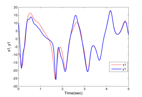
For simulation, the MATLAB is used to solve the differential equation of controlled error dynamical system (6), based on fourth-order Runge-Kutta scheme with time step 0.001 and the and the initial values of the drive system and the response system are following $( - 10 , - 5,0,10,20,10 )$ and $( 10,5,0 , - 10 , - 20,5 )$ respectively. We choose the parameters $= 10 , b = \frac { 8 } { 3 } , c = 28 , d = 2 , k = 8.4 , l = 1$ and $h = 1$.
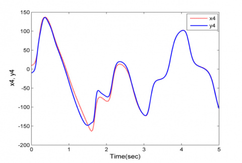
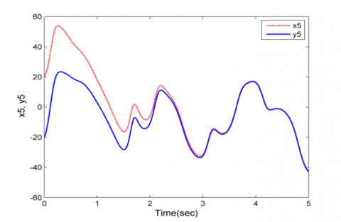
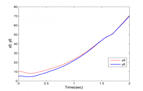
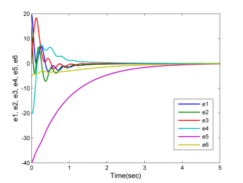
Figures 7-12 show the complete/full synchronization of the hyperchaotic Lorenz system (1) and system (4). Figure 13 shows the convergent for system (6) with controller (7).
Figure 7. Complete synchronization of the states $x _ { 1 }$ and $y _ { 1 }$ for the Lorenz systems (1) and (4)
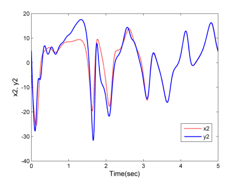
Figure 8. Complete synchronization of the states $x _ { 2 }$ and $y _ { 2 }$ for the Lorenz systems (1) and (4)
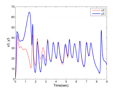
Figure 9. Complete synchronization of the states $x _ { 3 }$ and $y _ { 3 }$ for the Lorenz systems (1) and (4)
Figure 10. Complete synchronization of the states $x _ { 4 }$ and $y _ { 4 }$ for the Lorenz systems (1) and (4)
Figure 11. Complete synchronization of the states $x _ { 5 }$ and $y _ { 5 }$ for the Lorenz systems (1) and (4)
Figure 12. Complete synchronization of the states $x _ { 6 }$ and $y _ { 6 }$ for the Lorenz systems (1) and (4)
Figure 13. The convergent of the error dynamics (6) with controller (7)
In this article, controller was designed via the nonlinear control strategy for controlling of a 6-D hyperchaotic system based on the Lyapunov stability theory. Obviously from this controller, we achieved complete synchronization although this system is higher-dimensional hyperchaotic with unknown parameters and more complex from low-dimensional chaotic system. The effectiveness of these proposed control strategies was validated by numerical simulation results.
The authors thank the University of Mosul for support this research under the College of Computer Sciences and Mathematics
|
LE |
Lyapunov Exponents |
|
ei |
Error dynamics |
|
V(e) |
Lyapunov candidate function |
|
Greek symbols |
|
|
λi |
Roots of the characteristic equation |
|
Subscripts |
|
|
U p |
Control Matrix of Lyapunov function |
|
Q |
Matrix derivative of Lyapunov function |
[1] Chen, H.K. (2005). Global Chaos synchronization of new chaotic systems via nonlinear control. Chaos, Solitons and Fractals, 23: 1245-1251. https://doi.org/10.1016/j.chaos.2004.06.040
[2] AL-Azzawi, S.F. (2012). Stability and bifurcation of pan chaotic system by using Routh-Hurwitz and Gar-dan method. Appl. Math. Comput., 219: 1144-1152. https://doi.org/10.1016/j.amc.2012.07.022
[3] Al-Obeidi, A.S., AL-Azzawi, S.F. (2018). Complete synchronization of a novel 6-D hyperchaotic Lorenz system with known parameters. International Journal of Engineering & Technology, 7(4): 5345-5349. https://doi.org/10.14419/ijet.v7i4.18801
[4] Park, J.H. (2005). Chaos synchronization of a chaotic system via nonlinear control. Chaos Solitons Fractals, 25: 579-584. https://doi.org/10.1016/j.chaos.2004.11.038
[5] Liu, N., Gao, Q. (2018). Temperature prediction of oil well during circulation of compressible aerated fluids with leakage. Modelling, Measurement and Control B, 87(2): 92-96. https://doi.org/10.18280/mmc_b.870205
[6] Aziz, M.M., AL-Azzawi, S.F. (2016). Control and synchronization with known and unknown parame-ters. Appl. Math., 7: 292-303. http://dx.doi.org/10.4236/am.2016.73026
[7] Aziz, M.M., AL-Azzawi, S.F. (2017) Anti-synchronization of nonlinear dynamical systems based on Cardano’s method. Optik, 134: 109-120. https://doi.org/10.1016/j.ijleo.2017.01.026
[8] Al-Obeidi, A.S., AL-Azzawi, S.F. (2019). Projective synchronization for a class of 6-D hyperchaotic Lorenz system. Indonesian Journal of Electrical Engineering and Computer Science, 16(2): 692-700. https://doi.org/10.11591/ijeecs.v16.i2
[9] Aziz, M.M., AL-Azzawi, S.F. (2017). Hybrid chaos synchronization between two different hyperchaotic systems via two approaches. Optik, 138: 328-340. https://doi.org/10.1016/j.ijleo.2017.03.053
[10] Jia, Q. (2008). Hyperchaos synchronization between two different hyperchaotic systems. Journal of Information and Computing Science, 3: 73-80.
[11] Lu, D., Wang, A., Tian, X. (2008). Control and synchronization of a new hyperchaotic system with unknown parameters. International Journal of Nonlinear Science, 6: 224-229.
[12] Aziz, M.M., AL-Azzawi, S.F. (2015). Chaos control and synchronization of a novel 5-D hyperchaotic Lorenz system via nonlinear control. Int. J. Mode. Phys. Appli. 2: 110-115.
[13] Aziz, M.M., AL-Azzawi, S.F. (2017). Some problems of feedback control strategies and its treatment. Journal of Mathematics Research, 9(1): 39-49. https://doi.org/10.5539/jmr.v9n1p39
[14] AL-Azzawi, S.F., Aziz, M.M. (2018). Chaos synchronization of non-linear dynamical systems via a novel analytical approach. Alexandria Engineering Journal, 57(4): 3493-3500. https://doi.org/10.1016/j.aej.2017.11.017
[15] AL-Azzawi, S.F., Aziz, M.M. (2019). Strategies of linear feedback control and its classification. Telkomnika (Telecommunication, Computing, Electronics and Control, 17(4): 1931-1940. http://dx.doi.org/10.12928/telkomnika.v17i4.10989
[16] Yang, Q., Osman, W.M., Chen, C. (2015). A new 6D hyperchaotic system with four positive Lyapunov exponents coined. Int. J. Bifurcation and Chaos, 25(4): 1550061-1550079. https://doi.org/10.1142/S0218127415500601