Yan Lv* | Peng Zhang | Qiankun Hou | Xiaochen Li | Xueyu Zhang | Jialiang Sun | Xu Zhang | Xueheng Tao
OPEN ACCESS
In order to optimize the sensor arrays which are used to classify and identify these fluids. It preliminarily screens the response performance of single sensors in the testing system using the intra-class mean square, the F value and the P value by one-way analysis of variance (one-way ANOVA) meth-od, and then performs significance analysis of the screened sensors according to the multiple comparison analysis method, classify them by significance and then group them into three different sensor arrays. After that, this paper performs principal component analysis and cluster analysis on the signals of each sensor array, and the results show that the optimized sensor arrays all have better performance than the ones before optimization in classification and identification of samples, and that in particular, the optimized array I consisting of Au, Pt, Pd and W has the best performance and can be applied in the classification and identification of abalone flavoring liquids.
abalone flavoring liquid, one-way ANOVA, principal component analysis, optimization of sensor arrays
With the people’s living standards improving, the consumption de-mand for highly nutrient marine food such as abalone is also increas-ing. At present, abalone is mainly sold fresh in the market, and only few is made into frozen or dried products, which are not so popular among consumers as they are less nutrient and not so convenient to eat. Instant abalone, on the other hand, is quite popular in the market for its delicious taste, rich nutrition and convenient storage and trans-portation, etc. [1]. The taste of instant abalone is mainly controlled by the flavoring liquid during processing, which usually consists of water, salt, monosodium glutamate (MSG), vinegar, white sugar, bone soup, starch and spices, etc. With different types and amounts of the condi-ments, the instant abalone will taste differently. At present, the taste quality of abalone flavoring liquids is mainly subjectively evaluated by technicians with different personal conditions and physical health, and thus the results are not repeatable and also difficult to quantify [2]. Luckily, the electronic tongue is developed to address such problems. As a new type of artificial intelligence detection technology, it can identify and predict various liquid samples in a highly sensitive, re-peatable and reliable manner [3-8]. Therefore, it can also be applied in the taste prediction and detection of flavoring liquids in the production of instant abalone [9].
The electronic tongue detection technology mainly uses the sensor array and the pattern recognition algorithm to form a rapid detection system. The sensor is the basis for such an electronic tongue detection system. Considering the complex composition of the flavoring liquid, a large number of sensors are needed to obtain sufficient information to identify the substances as accurately as possible. However, due to the non-specificity and cross-sensitivity of the sensors, the collected information is significantly correlated. In addition, more sensors will also increase the noise interference and the difficulty of data pro-cessing. Therefore, it is necessary to optimize the sensor array [10-14].
This paper attempts to optimize the sensor arrays for detection of abalone flavoring liquids. It determines the stability and differences of sensors by the one-way ANOVA method and eliminate those with poor performance. Then it uses the multiple comparison analysis meth-od to obtain the significant differences between the remaining sensors, and classifies and group them into several different arrays. Through the principal component analysis in conjunction with the cluster analy-sis (Euclidean distance), this paper obtains the identification perfor-mance of several sensor arrays and selects the one with the best perfor-mance as the optimal sensor array for identification of abalone flavor-ing liquids.
2.1 Experimental materials
The abalone flavoring liquid is usually composed of salt (1%~3%), MSG (0.1%~0.5%), small amount of vinegar and other minor ingredi-ents. In selection of the samples for identification, if the samples have little difference in concentration, it will be difficult to distinguish them. Therefore, in this experiment, 5 samples with different concen-trations were prepared according to the difference thresholds of the three main ingredients in the common concentration ranges in the con-ditioning liquid [15, 16], respectively denoted as A, B, C, D and E (Table 1). The salt was supplied by Dalian Salt Industry Co., Ltd. (product standard No. GB 5461), vinegar by Dalian Seasoning Food Factory (product standard No. SB/T 10337) and MSG by Shenyang Hongmei Food Co., Ltd. (product standard No. GB/T 8967 ). The cor-responding taste substances were weighed according to the amounts specified in Table 1 and dissolved in 100 ml of deionized water to prepare samples. After being evenly mixed, all the samples were placed in a freezer for later use.
Table 1. Formulas of the abalone flavoring liquid samples with 5 different concentrations*
|
Sample number |
Salt content (g) |
MSG content (g) |
Vinegar content (ml) |
|
A |
1.286 |
0.782 |
2 |
|
B |
1.622 |
0.978 |
2.42 |
|
C |
2.043 |
1.222 |
2.94 |
|
D |
2.574 |
0.978 |
2 |
|
E |
3.243 |
1.222 |
2.42 |
|
*The content of each taste substance listed in the table refers to the mass of the substance contained in the deionized water per 100ml under the formula. |
|||
2.2 Experimental apparatuses
The CHI620E electrochemical analyzer was provided by Shanghai Chenhua Instrument Co., Ltd.; 6 kinds of metal disk electrodes (Au, Pd, Pt, Ni, W and Ag) with a diameter of 2mm were used as working electrodes, the R0303 Ag-AgCl electrode as the reference electrode, and the Pt010 Pt column electrode (φ1mm×10mm) as the auxiliary one, provided by Tianjin Ida Hengsheng Technology Co., Ltd.; the FA1004B electronic scale by Shanghai Yueping Scientific Instrument Co., Ltd.; the HJ-2 double-end magnetic heating stirrer by Changzhou Guohua Electric Appliance Co., Ltd.; the 202-series electric thermostat drying oven by Shanghai Shengke Instrument Equipment Co., Ltd.; the Haier BC/BD-102HT refrigerator by Qingdao Haier Co., Ltd.; and the KQ-2200DB ultrasonic cleaning machine by Kunshan Ultrasonic Instruments Co., Ltd.
2.3 Experimental method
The cyclic voltammetry was used as the excitation and acquisition method for the electrochemical signals of the sensor arrays, with the parameter settings shown in Table 2.
Table 2. Parameter settings for the voltammetry electrochemical analysis
|
Initial potential (V) |
High potential (V) |
Low potential (V) |
Scanning rate (V/s) |
Sampling interval (V) |
Sensitivity range |
|
-0.8 |
1.2 |
-0.8 |
0.1 |
0.001 |
e-5 ~e-3 |
In the electrochemical measurement based on cyclic voltammetry, the response curve of a sensor is a cyclic voltammogram formed as a result of the potential of the electrode under study being scanned from negative to positive. Before the experiment, the samples were taken out of the refrigerator, and placed at the ambient temperature of 22℃. 15min later, the experiment started. The samples were arranged according to the cyclic crossover sequence, that is, they were to be detected in the order of “A, B, C, D, E, A, B, C, D, E….”, to control the systematic error of the experiment [17].
2.4 Data processing and analytical method
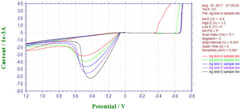
For each of the five concentrations of the flavoring liquid, three samples were prepared and each sample was repeatedly tested for five times. Figure 1 shows the cyclic volt-ampere response curves of the Ag electrode to the five different concentrations of flavoring fluid. The parameter Settings of cyclic voltammetry are shown in table 2. As shown in the figure that the shape of the curves are very similar and they have the biggest difference at the troughs. Usually, the peaks or troughs with certain stability in the response curve are selected as the feature points of the curve, which have a lower relative standard deviation (RSD) for the same sample, but can vary greatly for different samples [17]. The experiment selected the response peak current of each curve of the sensor under the signals excited by the cyclic volt-ampere potential as the measured value of one test, and thus obtained a 75×6 data matrix, where 6 refers to the signals of 6 sensors and 75 is the 75 groups of data obtained from 5 tests on each of the 3 samples for each of the 5 concentrations of the flavoring liquid. Firstly, the Grubbs method was used to exclude the abnormal data at a detection level of a=0.05. After the abnormal data were eliminated, the average of the repeated test values of each sample was taken as its eigenvalue, and a total of 15×6 pieces of data were obtained. In order to eliminate the dimensional differences in the sample test data between the sensors, the data were standardized by the Z-score standardization method. After the data were preprocessed, statistical analysis could be performed [18].
Figure 1. Response curves of the Ag electrode to the flavoring liquids with five different concentrations
In the one-way analysis of variance (one-way ANOVA), with each sensor as one factor and the response of each sample as a level, there was a 15×6 data matrix for ANOVA to screen the sensors and group the performances. After the sensor arrays were grouped, a 2D principal component score plot was obtained by the principal component analysis (PCA) method to compare the effects of the sensor arrays in distinguishing of the samples before and after optimization. PC1 and PC2 contained the contribution rates of the first and the second principal components obtained in the PCA transformation. The higher the cumulative contribution rate, the richer the sample information covered by the sensor array, and the better the identification performance of the sensor array with respect to the sample. Based on the principal component analysis, the inter-class Euclidean distances between the samples in the sensor principal component score plot were calculated to reflect the identification effect of the sensor array on each sample. According to the PCA and the Euclidean distance analysis results, the optimal sensor array was determined.
3.1 One-way ANOVA
The response performance of the sensors can directly affect the performance of the system. The stability of a sensor with respect to the same sample and whether it can discriminate the different samples are the main indicators of the response performance of the sensor [19]. In this experiment, according to the principle of the one-way ANOVA, the homogeneity test of variance was performed on the 15×6 data matrix with the sensor as one factor and the response signal eigenvalues of the 15 samples as the levels, to ensure that the data would met the ANOVA conditions. All sensors underwent one-way ANOVA using the data analysis software SPSS 22, and the results are shown in Table 3. The intra-class mean square value indicates the repeatability of the same sensor responding to the same sample. The smaller the mean square value, the better the repeatability of the sensor. The F value and the P value reflect the ability of the same sensor to distinguish between different samples. The larger the F value and the smaller the P value, the better the ability of the sensor to distinguish between the samples [19, 20].
Table 3. ANOVA results of the response performance of the sensors
|
Sensor name |
Mean square (Intra-class,´10-3) |
F value |
P value |
|
Au |
0.16 |
3627.21 |
2.76E-17 |
|
Pt |
2.58 |
1452.42 |
8.97E-14 |
|
Pd |
3.88 |
963.09 |
6.97E-13 |
|
Ag |
5.93 |
630.45 |
5.75E-12 |
|
Ni |
7.70 |
484.81 |
2.12E-11 |
|
W |
9.96 |
312.03 |
1.89E-10 |
It can be seen from Table 3 that the repeatability and distinguishing abilities of the Au, Pt, and Pd sensors were better than the Ag, Ni, and W ones, but that all the sensors had an intra-class mean square value less than 0.01 and a P value less than 0.05, indicating that all sensors had good repeatability and distinguishing abilities. To examine the significance of the differences between the sensors, the multiple comparison analysis method was performed. In such analysis, if the sensors are marked with the same letter, the differences between them are not significant, and if they are marked with different letters, it means there are significant differences between them [21]. The results are shown in Table 4.
Table 4. ANOVA results of the sensors by the multiple comparison analysis method
|
Sensor name |
Mean value |
5% significance level |
|
Pd |
0.975 |
a |
|
Pt |
1.116 |
b |
|
Au |
1.262 |
c |
|
Ni |
1.305 |
c |
|
Ag |
1.379 |
c |
|
W |
1.549 |
d |
As can be seen from Table 4, the Au, Ni, and Ag sensors did not have significant differences at a significant level of 5%. Therefore, each one of these three was selected in the optimization of a sensor array. In this way, the original 6 sensors were divided into 3 arrays, denoted as I, II and III. The combination of sensor array before and after optimization are shown in table 5, unoptimized array contains 6 sensors as Au, Pd, Pt, Ni, W and Ag, optimized array I contains the Au, Pd, Pt and W sensors, optimized array II contains the Ag, Pd, Pt and W sensors, and optimized array III contains the Ni, Pd, Pt and W sensors.
Table 5. Sensor array combination before and after optimization
|
Sensor array name |
Included sensor |
|
Unoptimized array |
Au, Pd, Pt, Ni, W, Ag |
|
Optimized array I |
Au, Pd, Pt ,W |
|
Optimized array II |
Ag, Pd, Pt ,W |
|
Optimized array III |
Ni, Pd, Pt ,W |
Table 6. PCA analysis results of the sensor arrays before and after optimization
|
Sensor array name |
Variance contribution rate of the first principal component (PC1) |
Variance contribution rate of the second principal component (PC2) |
Cumulative variance contribution rate of the first and second principal components (PC1+PC2) |
|
Unoptimized array |
77.65% |
17.46% |
95.11% |
|
Optimized array I |
83.29% |
14.17% |
97.46% |
|
Optimized array II |
82.29% |
13.45% |
95.74% |
|
Optimized array III |
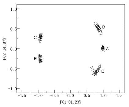
81.23% |
14.87% |
96.10% |
3.2 Principal component analysis (PCA)
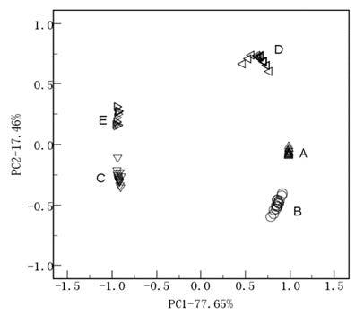
The original six sensor arrays were ones before optimization, and the three sensor arrays I, II, and III obtained through the above ANOVA are ones after optimization. In order to study the differences in the flavoring liquid identification performance of the sensor arrays before and after optimization, they were used to distinguish the flavoring liquids with five different concentrations, as shown in Table 1. Then the principal component analysis was performed on the 75×6-dimensional response data of the sensor arrays before optimization and the 75×4- dimensional response data of the optimized arrays I, II and III. The results are shown in Table 6, and the analysis charts are shown in Figure 2 to 5.
Figure 2. PCA analysis chart of the unoptimized array
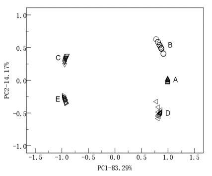
Figure 3. PCA analysis chart of the optimized array I
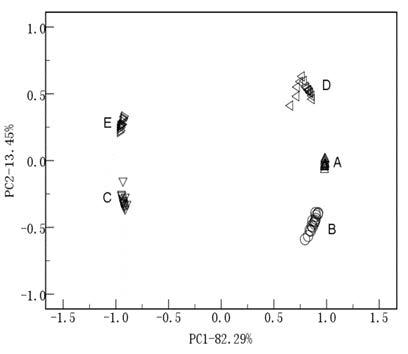
Figure 4. PCA analysis chart of the optimized array II
Figure 5. PCA analysis chart of the optimized array III
Through comparison of the PCA analysis results of the sensor arrays before and after optimization, it is found that for the optimized sensor arrays, not only did the cumulative variance contribution of the first principal component increase, but that those of the first two also in-creased, and that the optimized array I had the best result. Overall, the optimized sensor arrays can cover more sample information than the ones before optimization.
It can also be seen from the 2D PCA score charts that the optimized sensor arrays all had better abilities to distinguish the samples - the similar types of samples were distributed more closely and the different types were more disperse. On the basis of the PCA analysis, the Euclidean distance was further calculated for the score points. Then the extreme values of the Euclidean distances between the 15 samples before and after the optimization were compared for the differences in the sample clustering performance of the arrays. The results are shown in Table 7.
Table 7. Analysis results of the extreme values of the Euclidean distances given by sensor arrays before and after optimization
|
Sensor array name |
A |
B |
C |
D |
E |
|||||
|
Max (0.1) |
Min (0.1) |
Max (0.1) |
Min (0.1) |
Max (0.1) |
Min (0.1) |
Max (0.1) |
Min (0.1) |
Max (0.1) |
Min (0.1) |
|
|
Unoptimized array |
2.15 |
1.11 |
2.40 |
9.17 |
3.47 |
1.93 |
2.44 |
1.65 |
3.90 |
3.61 |
|
Optimized array I |
1.89 |
0.83 |
2.13 |
6.22 |
3.16 |
1.58 |
1.66 |
0.79 |
3.23 |
0.97 |
|
Optimized array II |
1.91 |
1.04 |
2.38 |
8.89 |
3.45 |
1.79 |
2.39 |
1.37 |
3.49 |
1.07 |
|
Optimized array III |
2.13 |
0.76 |
2.14 |
6.48 |
3.19 |
1.60 |
2.13 |
1.21 |
3.66 |
3.33 |
As shown in Table 7, the Euclidean distance of each of the five samples A, B, C, D and E before optimization was greater than that after optimization, indicating that the optimized sensor arrays were better than those before optimization in terms of the sample clustering performance. In particular, the optimized array I was better than II and III in terms of the clustering performance.
Through the above principal component analysis and the Euclidean distance calculation, it can be seen that the optimized array I was better than that before optimization in both the coverage and the clustering of the sample information. Therefore, the optimized array I (Au, Pt, Pd and W) was finally selected to identify the abalone flavoring liquids.
A sensor array consisting of 6 different metal electrodes was used to classify and identify the abalone flavoring liquids with 5 different con-centrations. Based on the sensor array signal data, the one-way ANO-VA, principal component analysis and clustering performance analysis were performed to select the optimal combination.
(1) In the one-way ANOVA, the intra-class mean square value, the F value and P value were used to determine whether a sensor could give repeatable response to the same sample and different responses to dif-ferent samples. On the premises that the requirements for repeatability and distinguishing ability were met, the sensors were subjected to mul-tiple comparison analysis and then combined into 3 arrays according to their significant differences.
(2) The PCA results show that the cumulative variance contributions of the first two principal components in the optimized sensor array increased, especially for optimized array I, where the cumulative vari-ance contributions of the first two principal components were the high-est – up to 97.466%. This indicates that the optimized array I has the best ability to distinguish between the samples.
(3) The results of clustering analysis were consistent with those of the principal component analysis-the optimized array I had better clus-tering performance than other ones, which further verifies the PCA results.
This study is funded by Natural Science Foundation of Liaoning Province (20180550454) and Public Science and Technology Research Funds Projects of Ocean(201505029).
[1] Y. Liu, J. Wang, J. F. Sun, J. Wang, Modern Food Science and Technology, 29(3), 673 (2013).
[2] X. T. Chen, J. N. Wu, H. X. Lu, Z. Y. Liu, Y. H. Chen, Food Sci-ence, 39(04), 282 (2018).
[3] J. J. Zhang, S. Q. Gu, Y. T. Ding, X. C. Wang, W. M. Jiang, Food Science, 36(4), 141 (2015).
[4] M. X. Wang, X. P. Bo, S. J. Han, J. H. Wang, B. Y. Han, Transac-tions of the Chinese Society of Agricultural Engineering, 32(16), 300 (2016).
[5] D. Chen, T. Ma, W. L. San, X. Wang, Q. D. Li, Food Science, 38(18), 168 (2017).
[6] H. Y. Yu, Y. Zhang, C. H. Xu, H. X. Tian, Transactions of the Chi-nese Society of Agricultural Engineering, 33(2), 297 (2017).
[7] M. Liu, S. M. Tan, H. L. Zhang, F. H. Liu, Food Science, 39(15), 88 (2018).
[8] N. Kishimoto, Chemical engineering transactions, 68, 301 (2018).
[9] X. L. Zhang, Y. Lv, H. H. Wang, X. H. Tao, X. Zhang, Carpathian Journal of Food Science & Technology, 8(2), 107 (2016).
[10] R. S. Kadam, A. Kulkarni, Traitement du Signal, 35(2), 153 (2018).
[11] Y. S. Miao, H. R. Wu, H. J. Zhu, Y. L. Song, Ingénierie des Sys-tèmes d’Information, 23(5), 69 (2018).
[12] V. Messina, M. Sance, G. Grigioni and N. W. D. Reca, IEEE Sen-sors journal, 14(6), 1756 (2014).
[13] L. S. B. Raguram, V. M. Shanmugam, Traitement du Signal, 34(3- 4), 137 (2017).
[14] S. Deshmukh, A. C. Romain, Chemical Engineering Transactions, 68, 343 (2018).
[15] S. P. Zhang, S. Y. Tian, S. P. Deng, Journal of Chinese institute of food science and technology, 9(5), 112 (2009).
[16] W. B. Zhang, “Food Sensory Scale Field Analysis:an Experimental and Theoretical Study of Gustatory Behavior”, Hang Zhou: Zhejiang Gongshang University, 2012.
[17] L. Zhao, B. L. Shi, H. Y. Wang, Z. Li, Food Science, 30(20), 367 (2009).
[18] P. Y. Yuan, Q. D. Meng, Y. Q. Jing, M. Zeng, Journal of Data Acquisition and Processing, 30(5), 1099 (2015).
[19] X. S. Zeng, D. W. Deng, L. Shi, G. H. Huang, Food Science, 34(12), 208 (2013).
[20] Z. N. Wang, L. M. Zheng, X. W. Fang, L. Yang, Meat Research, 29(5), 27 (2015).
[21] H. M. Zhang, J. Wang, Transactions of the Chinese Society of Agricultural Engineering, 22(12), 164 (2006).