Nitin K. Mishra![]() | Prerna Jain*
| Prerna Jain*![]() | Ranu
| Ranu![]()
© 2024 The authors. This article is published by IIETA and is licensed under the CC BY 4.0 license (http://creativecommons.org/licenses/by/4.0/).
OPEN ACCESS
This research introduces a decentralized supply chain optimization model that incorporates blockchain technology. The model, implemented through an optimized iterative method, integrates ordering, holding, and purchasing costs to offer a comprehensive view of total costs for both retailers and suppliers. The model's uniqueness and optimality are demonstrated through theoretical analysis, highlighting the optimal ordering interval as the sole solution to the derived equation. Employing an algorithmic methodology, optimal replenishment schedules are efficiently calculated using Wolfram Mathematica 13.0. A numerical example and sensitivity analysis illustrate the impact of key parameters on replenishment cycles, order quantity, and costs, encompassing wholesale prices, demand uncertainty, and holding/ordering costs. Managerial insights derived from sensitivity analysis guide decision-makers in optimizing supply chain management, emphasizing strategies such as wholesaler price balance and strategic blockchain information management. In essence, this research contributes to an enhanced understanding of decentralized supply chain models with blockchain, providing a systematic decision-making optimization approach for increased efficiency and resilience.
decentralized supply chain, blockchain technology, finite planning horizon, sensitivity analysis
The disruptive impact of COVID-19 underscores the vulnerability of centralized supply chain systems. Disruptions originating from a single source can have far-reaching consequences, impacting the global supply of goods and services. Decentralized supply chain models are emerging as robust solutions during this critical period [1, 2]. Through a multi-participant approach, these models distribute decision-making and resources among various participants, ensuring that a small issue in one part does not affect the entire system. In the aftermath of this pandemic, the flexibility, robustness, and power of a decentralized supply chain have become apparent, eliminating dependency on a single source.
In today's global business environment, supply chains have become increasingly complex and dispersed, leading to a need for better information sharing, visibility, and coordination among multiple stakeholders. The literature on decentralized supply chain models addresses the challenges and opportunities associated with managing these complex supply chains. Several studies have highlighted the importance of decentralized supply chain models in improving operational efficiency, reducing costs, and enhancing customer satisfaction. One key advantage of decentralized supply chain models is the greater autonomy they provide to individual subsidiaries or locations within a business [3].
In parallel, the advent of blockchain technology has transformed various industries by revolutionizing the storage and verification of transactions and data. One particular area where blockchain has shown great potential in the realm of supply chain management [4]. As supply chains become more complex and globalized, there is an increasing demand for innovative solutions that can improve traceability, efficiency, and transparency.
This research paper delves into the transformative journey of integrating Blockchain Technology into our decentralized supply chain. We aim to analyze the potential impact of this technology, especially within the finite planning horizon, to effectively manage our supply chain during disruptions [5]. Like a well-crafted recipe, this paper blends theory, case study, and practical insights, showcasing how blockchain can become a powerhouse for our decentralized supply chain. Together, feedback on a journey to explorer this new variant supply chain management, where innovative solutions powered by blockchain pave the way for a more liberated, silent, and efficient future.
In addition, this study incorporates quantitative analysis by employing numerical examples extracted from a secondary dataset compiled from a diverse array of [6, 7]. Our analysis is firmly grounded in a robust foundation. Utilizing an optimal iterative method, we systematically investigate the model's performance under varying wholesale prices. The primary objective is to contribute valuable insights into the optimization potential of the model across a spectrum of scenarios. This study not only extends the current body of research findings but also expands the examination of the model's behavior in response to diverse conditions of wholesale prices.
In this research paper, each section explains how blockchain technology enhances decentralized supply chain inventory models. Detailed literature reviews are presented in Section 2, including the impact of blockchain. Section 3 defines symbols and variables within the theoretical framework. We establish a theoretical framework and develop a model in this section. Section 4 explains the mathematical model for a blockchain-based supply chain inventory system. Literature challenges are addressed by the model, as well as its explained approach. A practical case study and numerical examples illustrate the model in Section 5. A sensitivity analysis is provided in Section 6, which evaluates the model's robustness under varying conditions, enabling optimization. This section offers supply chain decision-makers practical recommendations based on theoretical and numerical findings. Section 7 summarizes key findings, managerial implications, and future research directions.
Supply chain management is a dynamic field, and the exploration of decentralized supply chain models has revealed a multitude of approaches. Through an extensive review of existing research, various decentralized models were examined, shedding light on their respective contributions and limitations. Concurrently, a parallel investigation into blockchain technology's role in supply chain management unfolded, revealing a nascent utilization of this transformative technology. However, a noticeable gap emerged — the limited application of blockchain in decentralized supply chain models, prompting the need for a more comprehensive exploration. This literature review seeks to provide a coherent synthesis of these findings and identify avenues for bridging the research gap.
This literature review draws insights from a variety of supply chain models, each contributing to the understanding of decentralized decision-making and its impact on closed-loop supply chains. Huang et al. [8] investigate pricing decisions in a closed-loop supply chain under disruptions. Savaskan et al. [9] evaluate decentralized systems with a focus on product remanufacturing using a Stackelberg leadership model. Mungan et al. [10] investigate dual-channel supply chains, studying equilibrium conditions and the impact of factors like marginal costs. Dumrongsiri et al. [11] compare coordinated and decentralized decision-making for a monopolistic retailer facing time-varying demand. Chen and Chen [12] optimize procurement, production, and delivery schedules for technology-related companies. Li and Li [13] analyze analytical models related to active acquisition and remanufacturing in supply chains. Chen and Cheng [14] evaluate the price-dependent revenue-sharing mechanism in a decentralized supply chain using a Stackelberg game framework. Benkherouf et al. [15] determine optimal lot sizes for a recovery inventory system. Wu and Zhao [6] introduce a collaborative replenishment policy considering varying demand and check coordination between retailer and supplier. Yuan [16] develops a multi-period closed-loop supply chain model with remanufacturing. Bai et al. [17] analyze system coordination in a supply chain for deteriorating items using revenue-sharing contracts. Nagaraju et al. [18] developed a mathematical model for a three-echelon inventory system in both coordinated and non-coordinated supply chains. Giri et al. [19] investigate dual-channel supply chain models for selling deteriorating products. Liu et al. [20] establish a decision-making model under carbon tax constraints. Prasad et al. [21] compares total costs in decentralized and centralized supply chains. Mondal and Giri [22] explore the influence of Corporate Social Responsibility (CSR) efforts, and examine the impact of recycling and retailer fairness behaviour on a green supply chain. Kumar et al. [23] model and optimize a coordinated and non-coordinated three-echelon supply chain. Liu et al. [24] address coordination problems in closed-loop supply chains led by retailers, considering Stackelberg game theory. Huang et al. [8] develop a three-level supply chain model based on blockchain technology, emphasizing retailer sensitivity to information.
Blockchain technology has emerged as a pivotal force in revolutionizing supply chain management, offering multifaceted benefits across diverse dimensions. The study by Identify the transformative effects of blockchain on environmental efficiency in a multi-echelon supply chain in the study [25]. Dutta et al. [26] Conduct a comprehensive review of global and local supply chains to examine decentralized structures, consensus algorithms, and smart contracts. Based on simulation research, present a three-level supply chain model emphasizing blockchain's ability to reduce operational costs. "SmartRice," a sensor-based blockchain solution for addressing food value chain challenges, will be introduced by the study [27].
Decentralized supply chain models as well as blockchain applications in supply chain management reveal a distinct research gap around blockchain technology underutilization in enhancing decentralized supply chains. This gap becomes particularly relevant when inventory models are considered when planning over finite time horizons. A decentralized supply chain strategy needs to explore blockchain technology's untapped potential as shown by this gap. The study adopts a methodological approach that combines blockchain technology with models of decentralized supply chains to address this research gap. We explore inventory models within finite planning horizons to enhance the overall efficiency of supply chains through the optimization of decision-making processes.
Finally, the literature review provides a comprehensive overview of the decentralized supply chain landscape, examines the application of blockchain technology within supply chain management, and identifies an important research gap. We will provide insights into the transformative potential of blockchain technology in decentralized supply chain strategies in the following sections. To analyze the impact of blockchain technology on decentralized supply chain inventory models, a mathematical model was developed in this study. Within the context of a finite planning horizon, the model addresses key parameters and variables. Following this, iterative methods are used to solve the model, utilizing Wolfram Mathematica (13.0). With this methodology, the implications of blockchain technology are systematically examined. Decentralized supply chain management benefits from the combination of mathematical modeling and computational analysis because the conclusions are more accurate and reliable.
To develop the proposed model in this paper, we use the notations, assumptions and Boundary Conditions listed below.
3.1 Notations
|
$\alpha$ |
Amount of retailer information |
|
$\beta$ |
Coefficients that are sensitive to price |
|
$\theta$ |
A constant demand rate that is dependent on inventory levels. |
|
$\mu$ |
A proportion of the total retailers that are information-sensitive., where 0 ≤ $\mu$ ≤ 1 |
|
1−$\mu$ |
All other actors are not concerned with information |
|
k |
measure of how much it costs to share information |
|
d n |
Demand An integer that is less than zero that represents the number of times the inventory will be replenished during the planning horizon H |
|
W H C TC |
Wholesale price Finite planning horizon The purchasing cost per unit ($/unit) A cost estimate for the planning horizon H. |
|
Ss |
Setup cost of the supplier dollars per order |
|
Sr CB Ij+1(t) Qj+1 tj Tj+1 |
The ordering cost for the retailer dollars per order blockchain technology can provide retailers with a Huge amount of information at cost CB, where CB= kα At time 't', the inventory level in the 'j+1'th cycle' can be calculated, where 'j' is any integer between 0 and 'n-1' At time 't', the inventory level in the 'j+1'th cycle' can be calculated, where 'j' is any integer between 0 and 'n-1' jth replenishment time, where t0 = 0, tn = H The length of the replenishment cycle for the (j + 1)th time where j = 0, 1, 2, . .,n-1 |
3.2 Assumptions
3.3 Boundary conditions
The specified boundary conditions play a fundamental role in solving the associated differential equation, serving as essential constraints for our model. They serve to enhance the accuracy and reliability of our model by providing a well-defined framework, enabling precise simulation and analysis of the inventory system's dynamics within the finite planning horizon.
In the realm of Blockchain-based dynamics, recent studies such as [6-8] has shown that the real-time assessment of retailer demand depends on instantaneous stock levels. This complex relationship is expressed through the demand rate equation
$\begin{aligned} & D(t) \text { : }D(t)=(\mu \mathrm{d}+(1-\mu) d \alpha-\beta W) t+\theta I(t), \text { such that } \mathrm{t}_{\mathrm{i}} \leq \mathrm{t} \leq \mathrm{t}_{\mathrm{i}+1} \\ & \end{aligned}$ (1)
The inventory gradually depletes as the system goes through cycles expressed by a first-order linear differential equation:
$\begin{gathered}\frac{d}{d t} \mathrm{I}_{\mathrm{j}+1}(\mathrm{t})=-[\mu \mathrm{d}+(1-\mu) \mathrm{d} \alpha-\beta \mathrm{W}] \mathrm{t}-\theta \mathrm{I}_{\mathrm{j}+1}(\mathrm{t}), \,\mathrm{t}_{\mathrm{i}} \leq \mathrm{t} \leq \mathrm{t}_{\mathrm{i}+1}\end{gathered}$ (2)
Initial boundary values Ij +1(tj+1) = 0 & Ij+1 (tj) = θj+1
$\therefore$ linear first-order differential equation
$\Rightarrow$ Integrating factor: $e^{\int \theta \mathrm{dt}}=e^{\theta t}$
The subsequent exploration entails finding the solution to the differential equation, resulting in the order quantity for each cycle (Qj+1), and a complex representation of the total cost of retailer (TCR) equation that encompasses ordering, holding, and purchasing costs.
$\mathrm{I}_{\mathrm{j}+1}(\mathrm{t}) \cdot \mathrm{e}^{\theta \mathrm{t}}=\int-[\mu \mathrm{d}+(1-\mu) \mathrm{d} \alpha-\beta \mathrm{W}] t e^{\theta \mathrm{t}} \mathrm{dt}$ (3)
$\begin{aligned} & \mathrm{Q}_{\mathrm{j}+1}=\mathrm{I}_{\mathrm{j}+1}\left(\mathrm{t}_{\mathrm{j}}\right)=-\mathrm{e}^{-\theta \mathrm{t}} \int_{t_j}^{t_{j+1}}[\mu d+(1-\mu) d \alpha- \beta W] p e^{\theta p} d p \\ & \end{aligned}$ (4)
$\begin{gathered}\operatorname{TCR}\left(n, t_0, t_1, t_2, \ldots ., t_{n)}=\right. \sum_{j=0}^{n-1} h_r \int_{t_i}^{t_{j+1}} I_{j+1}(t) d t+\sum_{j=0}^{n-1} W Q_{j+1}+n S_r\end{gathered}$ (5)
$\mathrm{TCR}=\mathrm{nS}_{\mathrm{r}}+\sum_{\mathrm{j}=0}^{\mathrm{n}-1} \mathrm{~h}_{\mathrm{r}} \int_{\mathrm{t}_{\mathrm{j}}}^{\mathrm{t}_{\mathrm{j}+1}} \mathrm{e}^{-\theta \mathrm{t}} \mathrm{dt} \int_{\mathrm{t}_{\mathrm{j}}}^{\mathrm{t}_{\mathrm{j}+1}}-[\mu \mathrm{d}+(1-\mu) d \alpha-\beta W] p e^{\theta p d p}+\sum_{j=1}^{n-1} W \theta_{j+1}$
$\mathrm{TCR}=\mathrm{nS}_{\mathrm{r}}+\sum_{\mathrm{j}=0}^{\mathrm{n}-1} \mathrm{~h}_{\mathrm{r}} \int_{\mathrm{j}}^{\mathrm{t}_{\mathrm{j}+1}}[\beta \mathrm{W}-\mu \mathrm{d}-(1-\mu) d \alpha] p e^{\theta p_{d p}} \int_{t_j}^p e^{-\theta t} d t+\sum_{j=1}^{n-1} W \theta_{j+1}$ (6)
$\mathrm{TCR}=\mathrm{nS}_{\mathrm{r}}+\sum_{\mathrm{j}=0}^{\mathrm{n}-1} \mathrm{~h}_{\mathrm{r}} \int_{\mathrm{t}_{\mathrm{j}}}^{\mathrm{t}_{\mathrm{j}+1}}[\beta \mathrm{W}-\mu \mathrm{d}-(1-\mu) d \alpha] p e^{\theta p^{\prime}} d p\left[e \theta^{(p-t j)}-1\right]+\sum_{j=1}^{n-1} W Q_{j+1}$
$\operatorname{TCR}\left(\mathrm{n}, \mathrm{t}_0, \mathrm{t}_1, \mathrm{t}_2, \ldots \ldots \ldots \ldots, \mathrm{t}_{\mathrm{n}}\right)=\mathrm{nS}_{\mathrm{r}}+\sum_{\mathrm{j}=1}^{\mathrm{n}-1}\left(\frac{\mathrm{h}_{\mathrm{r}}}{\theta}+\right.\text { W) } \int_{t_j}^{t_{j+1}}[\beta W-\mu d-(1-\mu) d \alpha] e^{\theta\left(t-t_j\right)} d t-\frac{W}{\theta}[\beta W-\mu d-(1-\mu) d \alpha] \frac{H^2}{2}$ with $\mathrm{t}_0=0 \& \mathrm{t}_{\mathrm{n}}=\mathrm{H}.$
Retailers' replenishment policies determine the supplier's total costs. Thus, during the planning horizon H, his or her total costs are his or her setup cost and manufacturing cost.
$\begin{gathered}\operatorname{TCS}\left(n *, t *_0, t *_1, t *_2, \ldots \ldots, t *_{n *-1}\right)=n * S_s+ \sum_{j=0}^{n *-1} C Q *_{j+1}\end{gathered}$ (7)
Furthermore, during the planning horizon H, the total optimal order quantity is
$Q=\sum_{j=0}^{j=n *-1} Q_{j+1}^*$ (8)
To optimize a process, the aim is to minimize a specific Eq. (6) while keeping the value of ‘n’ constant. By taking the first partial derivative of the equation, we can obtain Eq. (9), which provides the optimal values for the ordering intervals, represented by tj. Once Eq. (9) is satisfied, it reveals these optimal values. By imposing certain constraints such as ‘t0=0’ & ‘tn=H’, the uniqueness of these optimal solutions is established and forms the basis for an efficient and effective model.
$\frac{\partial}{\partial t_j} \mathrm{TCR}\left(\mathrm{n}, \mathrm{t}_0, \mathrm{t}_1, \mathrm{t}_2, \ldots \ldots \ldots \ldots, \mathrm{t}_{\mathrm{n}}\right)=[\beta \mathrm{W}-\mu \mathrm{d}-(1-\mu) \mathrm{d} \alpha] \mathrm{t}_{\mathrm{j}}\left[e^{\theta\left(t_j-t_{j-1}\right)}-1\right]-\theta \int_{t_j}^{t_{j+1}}[\beta \mathrm{W}-\mu \mathrm{d}-(1-$ $\mu) \mathrm{d} \alpha]+e]^{\theta(t-\mathrm{tj})} \mathrm{dt}=0 .\mathrm{j}=1,2,3 \ldots, \mathrm{n}-1$. (9)
Let n*, t1*, t2*, ..., tn-1* represent the optimal solution for the Minimum TCR problem with parameters n, t, t1, t2, ..., tn.
Theorem 1: Uniqueness and Optimality interval
Consider a fixed parameter, n, and let Eq. (9) represent the total cost of retailer (TCR) function, in the context of supply chain optimization.
Proof: Our objective is to establish that the optimal ordering interval for this system is the unique solution to Eq. (9). To substantiate this claim, we delve into the properties of the Hessian matrix associated with TCR.
In comprehending the intricate relationship between replenishment cycles and times, we formulate key expressions. Notably,
$\begin{gathered}\frac{\partial^2 \mathrm{TC}_r^{\mathrm{IND}}\left(n_1, \mathrm{t}_0, \mathrm{t}_1, \mathrm{t}_2, \ldots \ldots, \mathrm{t}_n\right)}{\partial t_j^2}=(-\mathrm{W} \beta+\mathrm{d} \alpha(1-\mu)+\mathrm{d} \mu(W+\left.\frac{\mathrm{hr}}{\theta}\right)\left(e^{\theta\left(t_j-\mathrm{t}_{\mathrm{j}-1}\right)}-e^{\theta\left(t_{j+1}-t_j\right)}+e^{\theta\left(t_j-t_{j-1}\right)} \theta \mathrm{t}_j+\right.\left.e^{\theta\left(t_{j+1}-t_j\right)} \theta \mathrm{t}_{1-j}\right) \\ \frac{\partial^2 \mathrm{TC}_r^{\mathrm{IND}}\left(n_1, \mathrm{t}_0, \mathrm{t}_1, \mathrm{t}_2, \ldots \ldots \ldots, \mathrm{t}_n\right)}{\partial t_j \partial t_{j-1}}=-e^{\theta\left(t_j-\mathrm{t}_{\mathrm{j}-1}\right)} \theta(-\mathrm{W} \beta+d \alpha(1-\mu)+d \mu\left(W+\frac{h_r}{\theta}\right) t_j \\ \frac{\partial^2 \mathrm{TC}_r^{\mathrm{IND}}\left(n_1, \mathrm{t}_0, \mathrm{t}_1, \mathrm{t}_2, \ldots \ldots \ldots, \mathrm{t}_{n_1}\right)}{\partial t_j \partial t_{j+1}}=-e^{\theta\left(t_{j+1}-\mathrm{t}_j\right)} \theta(-\mathrm{W} \beta+d \alpha-\mu)+\frac{d \mu)\left(W+\frac{h_r}{\theta}\right) t_{1+j}}{\partial t_j \partial t_k}=0 \\ \text { and } \frac{\partial^2 \mathrm{TC}_r^{{I N D}}\left(n_1, \mathrm{t}_0, \mathrm{t}_1, \mathrm{t}_2, \ldots \ldots, \mathrm{t}_{n_1}\right)}{\partial t_j \partial t_k}=0\end{gathered}$
Furthermore,
$\begin{aligned} & \frac{\partial^2 T C_r^{I N D}\left(n_1, t_0, t_1, t_2, \ldots \ldots ., t_{n_1}\right)}{\partial t_j^2}>\left|\frac{\partial^2 T C_r^{I N D}\left(n_1, t_0, t_1, t_2, \ldots \ldots \ldots \ldots, t_n\right)}{\partial t_i \partial t_{j-1}}\right|+\left|\frac{\partial^2 T C_r^{I N D}\left(n_1, t_0, t_1, t_2, \ldots \ldots ., t_n\right)}{\partial t_j \partial t_{j+1}}\right| \text { for all } j=1,2, \ldots \ldots, n_1-1 .\end{aligned}$
Due to its diagonal properties, a Hessian matrix containing positive diagonal elements must also be positive definite. As a result, Eq. (9) has a unique solution which is the optimal replenishment interval as well as a global minimum value. If TCR is minimum, it must have a positive definite Hessian matrix r for a fixed n.
Proposition:
$t_{j+1} e^{\theta \mathrm{T}_{j+1}}<t_j\left(e^{\theta \mathrm{T}_j}+1\right)+\frac{1}{\theta} e^{\theta T_j}$
Proof: According to [13]:
$\mathrm{f}\left(\mathrm{t}_{j+1}\right)-\mathrm{f}\left(\mathrm{t}_j\right)<\frac{f^{\prime}\left(t_j\right)}{f\left(t_j\right)} \int_{t_j}^{t_{j+1}} f(u) d u$
We let $\mathrm{f}(\mathrm{t})=(\beta \mathrm{w}-\mu \mathrm{d}-(1-\mu) \mathrm{d} \alpha) \mathrm{t} e^{\theta\left(t-t_j\right)}$
Equation simplifies to
$\begin{gathered}{[\beta \mathrm{w}-\mu \mathrm{d}-(1-\mu) \mathrm{d} \alpha] \mathrm{t}_{j+1} e^{\theta\left(t_{j+1}-t_j\right)}-[\beta \mathrm{w}-\mu \mathrm{d}-(1-\mu) \mathrm{d} \alpha] \mathrm{t}_{\mathrm{j}}} \\ \left.\quad<\left(\theta+\frac{1}{t_j}\right) \int_{t_j}^{t_{j+1}} \beta w-\mu d-(1-\mu) d \alpha\right) t e^{\theta\left(t-t_j\right)} d t\end{gathered}$
Using Eq. (9) given by
$\begin{gathered}{[\beta \mathrm{w}-\mu \mathrm{d}-(1-\mu) \mathrm{d} \alpha] \mathrm{t}_{j+1} e^{\theta\left(t_{j+1}-t_j\right)}-[\beta \mathrm{w}-\mu \mathrm{d}-(1-\mu) \mathrm{d} \alpha] \mathrm{t}_{\mathrm{j}}}<\left(\theta+\frac{1}{t_j}\right)[\beta w-\mu d-(1-\mu) d \alpha] t_j e^{\theta\left(t_j-t_{j-1}\right)} \\ t_{j+1} e^{\theta \mathrm{T}_{j+1}}-t_j<\left(\theta+\frac{1}{t_j}\right) \frac{t_j e^{\theta T_j}}{\theta} \\ t_{j+1} e^{\theta \mathrm{T}_{j+1}}<\left(\theta+\frac{1}{t_j}\right) \frac{t_j e^{\theta T_j}}{\theta}+t_j \\ t_{j+1} e^{\theta \mathrm{T}_{j+1}}<e^{\theta T_j}+\frac{1}{\theta} e^{\theta T_j}+t_j\end{gathered}$
This leads to the conclusive result:
$t_{j+1} e^{\theta \mathrm{T}_{j+1}}<t_j\left(e^{\theta \mathrm{T}_j}+1\right)+\frac{1}{\theta} e^{\theta T_j}$
Lemma:
The monotonicity of tj (where j = 1, 2, …, n - 2) is evident concerning the parameter tn - 1. This lemma establishes the consistent increase of tj concerning the penultimate time point in the planning horizon.
Proof: The equation is simplified using the relationship Tn = H - tn-1 is constant if tn-1 is known, as per [15] say.
This implies that Tn and tn-1 are inversely related.
To prove that rate of change of TCR’s increase with Tn for j= n-1, n-2,…,3,2,1.
For j = n - 1, after differentiating Eq. (9) w.r.t. Tn, we get,
$\begin{gathered}\mathrm{TCR}=[\beta \mathrm{w}-\mu \mathrm{d}-(1-\mu) \mathrm{d} \alpha]\left[(-1) e^{\theta \mathrm{T}_{n-1}}+(H-\right.\left.\left.T_n\right) e^{\theta \mathrm{T}_{n-1}} \frac{\mathrm{dT}_{n-1}}{\mathrm{dT}_n}-t_n e^{\theta \mathrm{T}_n} \cdot \theta+e^{\theta \mathrm{T}_n} \cdot \theta\right]=0 \\ t_n e^{\theta \mathrm{T}_n} \cdot \theta=e^{\theta \mathrm{T}_n} \cdot \theta-e^{\theta \mathrm{T}_{n-1}}+\left(H-T_n\right) e^{\theta \mathrm{T}_{n-1}} \frac{\mathrm{dT}_{n-1}}{\mathrm{dT}_n}\end{gathered}$
Using preposition and Eq. (9) we get
$\begin{gathered}e^{\theta \mathrm{T}_n} \cdot \theta-e^{\theta \mathrm{T}_{n-1}}+\left(H-T_n\right) e^{\theta \mathrm{T}_{n-1}} \frac{\mathrm{dT}_{n-1}}{\mathrm{dT}}>\theta \mathrm{t}_{n-1}\left(e^{\theta \mathrm{T}_{n-1}}+\right.\text { 1) }+e^{\theta \mathrm{T}_{n-1}} \frac{d T_{n-1}}{d T_n}>0\end{gathered}$
Inequality concludes that
$\frac{d T_{n-1}}{d T_n}>0$
Indicating an increase in tn-1 as Tn increases. A generalization is made, suggestion that this relationship holds for j= n-1, n-2,…,3,2,1 and can be reasonably extended.
Expanding on the established formulations, we can apply the subsequent optimization procedure to uncover the most advantageous values and outcomes. The methodology involves an iterative optimization process, commencing with the practical decision to set 'n' to 2 as the initial point. When n = 1, we assign t0 = 0 and t1 = 4, and then initiate the Mathematica program to solve for optimality. For n = 2, corresponding to the number of replenishment cycles, where t0 = 0 and t2 = 4, the value of t1 is determined using an iterative method in the Mathematica program.
5.1 Methodology
The retailer should determine the most efficient way to schedule orders.
5.2 Numerical example
Using the assumptions in Section 3, this numerical example shows how changes in the key parameter value W affect the optimal results.
EXAMPLE- Given $\alpha=\beta=5, \mu=0.40, \mathrm{C}=\$ 12 /$ unit, $\mathrm{d}=$ 120/unit, $\mathrm{Ss}=\$ 120$ /setup, $\mathrm{Sr}=\$ 90 /$ order, $\mathrm{hr}=\$ 2 /$ unit/year, $\theta=0.75, \mathrm{H}=4$-year, $\mathrm{d}=120$ units/year, $\mathrm{W}=10,20,30$ units/year, respectively.
The results are shown in Tables 1-2 because of the algorithm and its corresponding expressions.
Table 1. Total cost for retailer when
|
$\mathbf{W} \rightarrow \mathbf{n}$ |
1 |
2 |
3 |
4 |
5 |
6 |
|
10 |
38025 |
36978 |
36944 |
36881 |
36898 |
36948 |
|
20 |
56913 |
56308 |
56478 |
56440 |
56468 |
56256 |
|
30 |
67948 |
67694 |
68117 |
67993 |
68032 |
68096 |
Table 2. Replenishment time for TCR, TCS, and Q
|
$\rightarrow \mathbf{t}_{\mathbf{i}} \mathbf{W}$ |
t1 |
t2 |
t3 |
t4 |
n |
TCR |
TCS |
Q |
|
10 |
1.105 |
1.961 |
2.704 |
4 |
4 |
36681 |
34370 |
2866 |
|
20 |
1.604 |
4 |
|
|
2 |
56308 |
29603 |
2446 |
|
30 |
1.604 |
4 |
|
|
2 |
67694 |
24836 |
2049 |
Maintaining a consistent value for 'n' ensures uniformity throughout the analysis, thereby facilitating a fair comparison across diverse iterations of the model. The provided table delineates the retailer's total cost for varying values of 'W' (wholesale price) and 'n' (replenishment cycles). The steadfastness in 'n' simplifies the assessment of how different wholesale prices influence the total cost over an identical number of replenishment cycles.
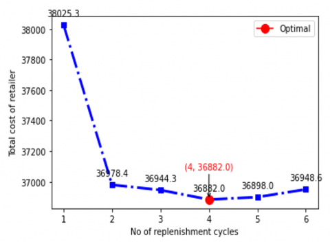
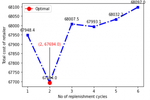
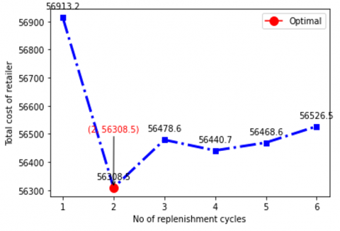
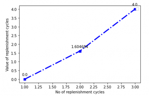
(a) n = 4
(b) n = 2
(c) n = 2
Figure 1. Optimal values of total cost of retailer and replenishment cycles
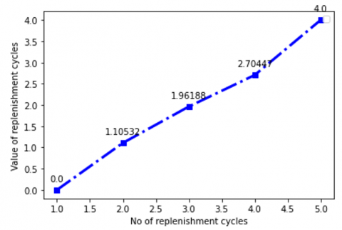
(a) n = 4
(b) n = 2
Figure 2. Increased order of optimal values of the replenishment cycles
The iterative process involves adjusting 'n' based on the comparison of total costs (TCR), aiming for convergence toward the optimal ordering policy. This iterative refinement is pivotal for attaining the most effective solution, allowing researchers to converge toward the configuration that minimizes total retailer costs. The algorithm's termination condition, highlighted in the table, dictates halting when the TCR for 'n' is less than TCR for 'n-1'.
Maintaining a consistent value for 'n' ensures uniformity throughout the analysis, thereby facilitating a fair comparison across diverse iterations of the model. The provided table delineates the retailer's total cost for varying values of 'W' (wholesale price) and 'n' (replenishment cycles). The steadfastness in 'n' simplifies the assessment of how different wholesale prices influence the total cost over an identical number of replenishment cycles.
The iterative process involves adjusting 'n' based on the comparison of total costs (TCR), aiming for convergence toward the optimal ordering policy. This iterative refinement is pivotal for attaining the most effective solution, allowing researchers to converge toward the configuration that minimizes total retailer costs. The algorithm's termination condition, highlighted in the table, dictates halting when the TCR for 'n' is less than TCR for 'n-1'.
For instance, when 'W' is 10 and 'n' is 2, the retailer's total cost amounts to 36978. With an incremental increase in 'n' from 2 to 6, the total cost fluctuates, culminating in its nadir at 'n' equals 4, registering a cost of 36881. This illustrates how the iterative process systematically refines 'n' to pinpoint the optimal ordering policy within defined constraints.
To visually comprehend these fluctuations, refer to Figure 1(a), which illustrates how values oscillate and reach their lowest point at 'n' equals 4. The same insights are conveyed for different 'W' values in both Table 1 and the Figure 1(b) and (c).
In Table 2 the intricate details of optimal outcomes in scenarios where compensation is factored into each optimal case. It can be rigorously established that the inequality tj+1 - tj < tj - tj-1 holds true, where j=1, 2,…,n−1. Here, tj denotes the jth replenishment time, with t0=0 and tn−1= H, where H is a non-negative integer.
Table 2 meticulously tabulates values for tj (replenishment time), Total Cost of Replenishment (TCR), Total Cost of Setup (TCS), and Order Quantity (Q). This tabulation distinctly delineates how diverse W (wholesale prices) correlate with specific tj values, thereby accurately characterizing optimal ordering policies for our model. For instance, when W is set at 10, t1 assumes a value of 1.105, t2 registers as 1.961, t3 stands at 2.704, and t4 reaches 4. Additionally, TCR manifests as 36681, TCS as 34370, and Q as 2866.
This illustrative example underscores the dynamic interplay of optimal replenishment times, costs, and order quantities across distinct W values. It underscores the adaptive nature of our model, optimizing parameters and enabling judicious decision-making to foster cost-effectiveness in the supply chain. Complementing the tabulated values in Table 2, our analysis extends to scrutinizing tj values, symbolizing replenishment time, elucidated through Figure 2(a) and (b).
In these graphical representations, the discernible convexity of the curve, influenced by tj fluctuations, serves as a visual indicator of optimal cycle points and cost minimization. This visual inspection of tj values enriches our understanding of the nuanced shifts in our model's performance, empowering strategic decision-making to optimize the intricacies of the supply chain.
6.1 Sensitivity analysis
In this section, we will conduct sensitivity analysis, by introducing percentage changes, our objective is to ensure that our model operates effectively within its predefined domain, rather than being adversely affected by alterations in the vicinity of any specific parameter. Additionally, this analysis provides valuable insights into the behavior of all parameters, facilitating the extraction of managerial insights. We have deliberately selected these specific percentages to comprehensively explore both sides of the function's domain, enabling a thorough study of the model's behavior.
Firstly, alterations in the Wholesale Price (W) wield substantial influence; (Table 3) a 20% decrease in W amplifies optimal replenishment cycles, order quantities, and overall cost for both suppliers and retailers. A 10% decrease a comparable effect, less pronounced, while a constant W (0%) maintains unaltered optimal values. Conversely, a 10% increase in W prompts a reduction in the optimal replenishment cycle, cost, and order quantity, with a more pronounced impact from a 20% increase. Moving on to Demand Uncertainly, a 20% reduction results in diminished orders and costs for both retailers and suppliers and a 10% reduction echoes a similar yet milder effect. Stable demand uncertainty (0% change) maintains consistent optimal values, but a 10% increase amplifies the total cost and quantity of the order. Doubling demand uncertainty (20% increase) leads to a significant upswing in optimal values. The parameters of Holding and Ordering Costs (α and β) exhibit their sway as a 20% reduction translates to diminished total order quantities and costs for retailers and suppliers. A 10% reduction yields a comparable albeit less prominent effect, while a steady state (0% change) preserves unaltered optimal values. Meanwhile, a 10% increase in α and β escalates total costs and order quantity, and a 20% increase brings similar results, albeit with higher optimal values. Shifting focus to the Unit Cost of the Product (d), a 20% reduction proves advantageous, diminishing total order quantities and costs for both retailers and suppliers. A 10% reduction yields a similar effect, albeit less pronounced, and a steady d (0% change) maintains consistent optimal values. Conversely, a 10% increase in d increases order quantity and costs, with a more dramatic surge resulting from a 20% increase. Finally, parameters such as hr, θ, Sr, Ss, and Cr exhibit minimal impacts on retailer and supplier cost estimates. These nuanced insights provide valuable guidance for managerial decision-making in optimizing the supply chain under varying conditions.
Table 3. Sensitivity analysis for each parameter
|
Paramters (P) |
% Changes |
Optimal Replenishment Cycle |
Total Order Quantity (Q) |
Total Cost of Retailer (TCR) |
Total Cost of Supplier (TCS) |
|
W |
-20 -10 0 10 20 |
2 2 2 2 2 |
2288.06 2168.89 2049.72 1930.55 1811.38 |
61816.08 65112.55 67694.00 69560.43 70711.84 |
27696.76 26266.72 24836.68 23406.64 21976.60 |
|
µ |
-20 -10 0 10 20 |
2 2 2 2 2 |
2354.79 2202.26 2049.72 2306.23 1744.64 |
77742.60 72718.30 67694.00 62669.70 57645.40 |
28497.58 26667.13 24836.68 23006.23 21175.78 |
|
α |
-20 -10 0 10 20 |
2 2 2 2 2 |
2288.06 2168.89 2049.73 1930.55 1811.38 |
75544.46 71619.23 67694.00 63768.77 59843.53 |
27696.76 23266.72 24836.68 23406.64 21976.60 |
|
β |
-20 -10 0 10 20 |
2 2 2 2 2 |
2288.06 2168.89 2049.73 1930.55 1811.38 |
75544.46 71619.23 67694.00 63768.77 59843.53 |
27696.76 23266.72 24836.68 23406.64 21976.60 |
|
d |
-20 -10 0 10 20 |
2 2 2 2 2 |
1401.43 1725.58 2049.72 2373.86 2698.00 |
46340.73 57017.37 67694.00 78370.63 89047.27 |
17057.26 20946.97 24836.68 28726.39 32616.10 |
|
hr |
-20 -10 0 10 20 |
2 2 2 2 2 |
2049.72 2049.72 2049.72 2049.72 2049.72 |
66489.54 67091.77 67694.00 68296.23 68898.46 |
24836.68 24836.68 24836.68 24836.68 24836.68 |
|
θ |
-20 -10 0 10 20 |
1 1 1 6 6 |
1307.11 1460.50 1633.34 1705.55 1746.84 |
58446.08 64349.82 71130.98 72948.19 74342.70 |
17706.05 18842.83 20069.88 21509.35 23072.50 |
|
Sr |
-20 -10 0 10 20 |
2 2 2 2 2 |
2049.72 2049.72 2049.72 2049.72 2049.72 |
67658.00 67676.00 67694.00 67712.00 67730.00 |
24836.68 24836.68 24836.68 24836.68 24836.68 |
|
Ss |
-20 -10 0 10 20 |
2 2 2 2 2 |
2049.72 2049.72 2049.72 2049.72 2049.72 |
67694.00 67694.00 67694.00 67694.00 67694.00 |
24788.68 24812.68 24836.68 24860.68 24884.68 |
|
d |
-20 -10 0 10 20 |
2 2 2 2 2 |
2049.72 2049.72 2049.72 2049.72 2049.72 |
67694.00 67694.00 67694.00 67694.00 67694.00 |
19917.34 22377.01 24836.68 27296.35 29756.02 |
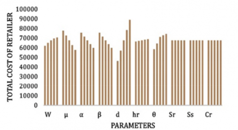
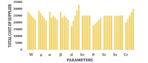
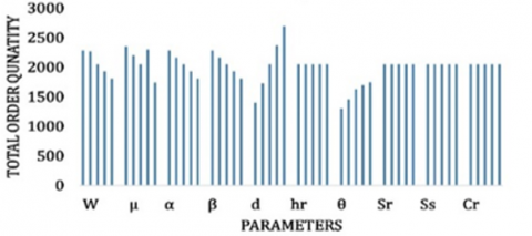
6.2 Managerial insights
In delving deeper into the sensitivity analysis, it becomes evident that various parameters have diverse impacts on the overall cost structure. The Wholesale Price (W) holds substantial significance, directly influencing cost structures for both retailers and suppliers shown in Figure 3(a) and (b). Changes in W affect order quantities, replenishment cycles, and overall costs, with higher prices leading to reduced order quantities and increased costs. The Demand Uncertainty (µ) significantly affects orders and costs, emphasizing the need for efficient information-sharing practices to mitigate rising retailer costs (shown in Figure 3(a)) associated with increased uncertainty (higher µ).
Holding and Ordering Costs (α and β) play a pivotal role in determining total order quantities and in (Figure 3) costs shown. Reductions in α and β lead to diminished order quantities and costs, underscoring the importance of efficient processes and strategic management in minimizing overall costs. The Unit Cost of the Product (d) directly influences order quantities and costs, demonstrating the sensitivity of the model to variations in unit cost.
On the other hand, parameters such as hr, θ, Sr, Ss, and Cr exhibit minimal impacts as shown in (Figure 3), suggesting their nuanced influence on overall cost structures. These parameters have relatively lower effects on key outcomes compared to other influential factors. Understanding these differential impacts provides valuable insights for managerial decision-making, highlighting critical factors that require strategic attention for achieving cost-effective supply chain management. Managers should focus on optimizing parameters with significant impacts, such as wholesale prices, demand uncertainty, and holding/ordering costs, to navigate the complexity of supply chain dynamics effectively. Meanwhile, parameters with minimal impacts may require less attention in strategic decision-making processes.
(a) Total cost of retailer
(b) Total cost of supplier
(c) Total order quantity
Figure 3. Sensitivity analysis
In conclusion, this research paper explores the transformative impact of integrating Blockchain Technology into decentralized supply chain models. The backdrop of the COVID-19 pandemic highlighted the vulnerabilities of centralized supply chain systems, leading to a growing recognition of the robustness and flexibility offered by decentralized models. Through a multi-participant approach, decentralized supply chain distributes decision-making and resources, reducing the risk of disruptions from a single source.
The literature review reveals a gap in the application of blockchain technology within decentralized supply chain models, particularly concerning inventory management over finite time horizons. This research addresses this gap by developing a mathematical model that integrates blockchain technology into the decision-making processes of decentralized supply chains.
The proposed model, based on a set of assumptions and notations, considers various parameters such as information sensitivity, demand rate coefficients, and setup costs. The mathematical formulation involves a first-order linear differential equation expressing the depletion of inventory over replenishment cycles. The cost for the retailer (TCR) equation encompasses ordering, holding, and purchasing costs, providing a comprehensive view of the financial implications.
The uniqueness and optimality of the replenishment interval are established through the analysis of the Hessian matrix associated with TCR, ensuring a global minimum value. The dynamic ordering interval inequality and the monotonic increase of replenishment cycles further contribute to the understanding of the understanding of the system’s behavior.
The methodology involves the optimization of the process by minimizing the TCR equation while keeping the value of ‘n’ constant. The numerical example demonstrates the sensitivity of the total costs and replenishment times to change in the blockchain-based wholesale price (W). The results emphasize the practical implications for supply chain optimization and decision-making.
The sensitivity analysis explores the impacts of different percentage changes in key parameters, providing valuable insights for managerial decision-making. Wholesale prices, demand uncertainty holding and ordering costs, and the unit cost of the product exhibit varying influences on optimal values, offering guidance for decision-makers under different conditions.
In summary, this research contributes to the understanding of how blockchain technology can enhance decentralized supply chain inventory models. The proposed model, along with its analysis and numerical examples, provide a foundation for future research and practical implementation. As supply chains continue to evolve, embracing innovative solutions powered by blockchain can pave the way for a more resilient, efficient, and transparent future.
Looking ahead, we envision extending this model to a three-echelon supply chain, fostering a comprehensive understanding of its dynamics. Future studies could explore variations in different time periods, uncovering additional nuances and enhancing the model’s applicability. As supply chains undergo transformations, the adoption of innovative blockchain-powered solutions holds the potential to foster a future characterized by enhanced resilience, efficiency, and transparency. Our research lays the groundwork for ongoing exploration in this realm, aligning with the overarching objective of promoting effective supply chain management.
[1] Haque, M., Paul, S.K., Sarker, R., Essam, D. (2022). A combined approach for modeling multi-echelon multi-period decentralized supply chain. Annals of Operations Research, 315(2): 1665-1702. https://doi.org/10.1007/s10479-021-04121-0
[2] Zhou, X., Tian, J., Wang, Z., Yang, C., Huang, T., Xu, X. (2022). Nonlinear bilevel programming approach for decentralized supply chain using a hybrid state transition algorithm. Knowledge-Based Systems, 240: 108119. https://doi.org/10.1016/j.knosys.2022.108119
[3] Algorri, M., Abernathy, M.J., Cauchon, N.S., Christian, T.R., Lamm, C.F., Moore, C.M.V. (2022). Re-Envisioning pharmaceutical manufacturing: Increasing agility for global patient access. Journal of Pharmaceutical Sciences, 111(3): 593-607. https://doi.org/10.1016/j.xphs.2021.08.032
[4] Omar, I.A., Debe, M., Jayaraman, R., Salah, K., Omar, M., Arshad, J. (2022). Blockchain-based supply chain traceability for COVID-19 personal protective equipment. Computers & Industrial Engineering, 167: 107995. https://doi.org/10.1016/j.cie.2022.107995
[5] Park, A., Li, H. (2021). The effect of blockchain technology on supply chain sustainability performances. Sustainability, 13(4): 1726. https://doi.org/10.3390/su13041726
[6] Wu, C., Zhao, Q. (2014). Supplier-retailer inventory coordination with credit term for inventory-dependent and linear-trend demand. International Transactions in Operational Research, 21(5): 797-818. https://doi.org/10.1111/itor.12060
[7] Mishra, N.K., Ranu. (2023). A supply chain inventory model for a deteriorating material under a finite planning horizon with the carbon tax and shortage in all cycles. Journal Européen des Systèmes Automatisés, 56(2): 221-230. https://doi.org/10.18280/jesa.560206
[8] Huang, Z., Shao, W., Meng, L., Zhang, G., Qiang, Q. P. (2022). Pricing decision for a closed-loop supply chain with technology licensing under collection and remanufacturing cost disruptions. Sustainability, 14(6): 3354. https://doi.org/10.3390/su14063354
[9] Savaskan, R. C., Bhattacharya, S., Van Wassenhove, L. N. (2004). Closed-loop supply chain models with product remanufacturing. Management Science, 50(2): 239-252. https://doi.org/10.1287/mnsc.1030.0186
[10] Mungan, D., Yu, J., Sarker, B.R. (2010). Manufacturing lot-sizing, procurement and delivery schedules over a finite planning horizon. International Journal of Production Research. https://doi.org/10.1080/00207540902878228
[11] Dumrongsiri, A., Fan, M., Jain, A., Moinzadeh, K. (2008). A supply chain model with direct and retail channels. European Journal of Operational Research, 187(3): 691-718. https://doi.org/10.1016/j.ejor.2006.05.044
[12] Chen, L.T., Chen, J.M. (2008). Optimal pricing and replenishment schedule for deteriorating items over a finite planning horizon. International Journal of Revenue Management, 2(3): 215. https://doi.org/10.1504/IJRM.2008.020622
[13] Li, X., Li, Y. (2011). Supply chain models with active acquisition and remanufacturing. Supply Chain Coordination Under Uncertainty, Springer, Berlin, Heidelberg, pp. 109-128. https://doi.org/10.1007/978-3-642-19257-9_5
[14] Chen, J.M., Cheng, H.L. (2012). Effect of the price-dependent revenue-sharing mechanism in a decentralized supply chain. Central European Journal of Operations Research, 20(2): 299-317. https://doi.org/10.1007/s10100-010-0182-3
[15] Benkherouf, L., Skouri, K., Konstantaras, I. (2014). Optimal lot sizing for a production-recovery system with time-varying demand over a finite planning horizon. IMA Journal of Management Mathematics, 25(4): 403-420. https://doi.org/10.1093/imaman/dpt015
[16] Yuan, J. (2015). Decision models of multi periods closed loop supply chain with remanufacturing under centralized and decentralized decision making. International Journal of U- and e-Service, Science and Technology, 8(10): 247-254. https://doi.org/10.14257/ijunesst.2015.8.10.24
[17] Bai, Q., Chen, M., Xu, L. (2017). Revenue and promotional cost-sharing contract versus two-part tariff contract in coordinating sustainable supply chain systems with deteriorating items. International Journal of Production Economics, 187: 85-101. https://doi.org/10.1016/j.ijpe.2017.02.012
[18] Nagaraju, D., Rao, A.R., Narayanan, S. (2016). Centralised and decentralised three echelon inventory model for optimal inventory decisions under price dependent demand. International Journal of Logistics Systems and Management, 23(2), 147. https://doi.org/10.1504/IJLSM.2016.073966
[19] Giri, B.C., Mondal, C., Maiti, T., Maiti, T. (2018). Analysing a closed-loop supply chain with selling price, warranty period and green sensitive consumer demand under revenue sharing contract. Journal of Cleaner Production. https://doi.org/10.1016/j.jclepro.2018.04.092
[20] Liu, Z., Hu, B., Zhao, Y., Lang, L., Guo, H., Florence, K., Zhang, S. (2020). Research on intelligent decision of low carbon supply chain based on carbon tax constraints in human-driven edge computing. IEEE Access, 8: 48264-48273. https://doi.org/10.1109/ACCESS.2020.2978911
[21] Prasad, T.V.S.R.K., Srinivas, K., Srinivas, C. (2020). Investigations into control strategies of supply chain planning models: A case study. Opsearch, 57(3): 874-907. https://doi.org/10.1007/s12597-020-00460-x
[22] Mondal, C., Giri, B.C. (2022). Investigating a green supply chain with product recycling under retailer’s fairness behavior. Journal of Industrial and Management Optimization, 18(5): 3641. https://doi.org/10.3934/jimo.2021129
[23] Kumar, P., Sharma, D., Pandey, P. (2022). Three-echelon apparel supply chain coordination with triple bottom line approach. International Journal of Quality & Reliability Management, 39(3): 716-740. https://doi.org/10.1108/IJQRM-04-2021-0101
[24] Liu, Y., Xia, Z.J., Shi, Q.Q., Xu, Q. (2021). Pricing and coordination of waste electrical and electronic equipment under third-party recycling in a closed-loop supply chain. Environment, Development and Sustainability, 23(8): 12077-12094. https://doi.org/10.1007/s10668-020-01158-2
[25] Manupati, V.K., Schoenherr, T., Ramkumar, M., Wagner, S.M., Pabba, S.K., Singh, R.I.R. (2020). A blockchain-based approach for a multi-echelon sustainable supply chain. International Journal of Production Research, 58(7): 2222-2241. https://doi.org/10.1080/00207543.2019.1683248
[26] Dutta, P., Choi, T.-M., Somani, S., Butala, R. (2020). Blockchain technology in supply chain operations: Applications, challenges and research opportunities. Transportation Research Part E: Logistics and Transportation Review, 142: 102067. https://doi.org/10.1016/j.tre.2020.102067
[27] Ekawati, R., Arkeman, Y., Suprihatin, Sunarti, T. C. (2022). Implementation of Ethereum blockchain on transaction recording of white sugar supply chain data. Indonesian Journal of Electrical Engineering and Computer Science, 29(1): 396. https://doi.org/10.11591/ijeecs.v29.i1.pp396-403