Sulaf Waiss*![]() | Ayad M. Dalloo
| Ayad M. Dalloo![]()
© 2024 The authors. This article is published by IIETA and is licensed under the CC BY 4.0 license (http://creativecommons.org/licenses/by/4.0/).
OPEN ACCESS
Most laser diodes experience fluctuations in intensity, phase, and wavelength, predominantly due to heating from energy conversion to thermal energy and changing ambient temperatures. This study primarily focuses on countering the effects of temperature variations through the design and implementation of a laser diode temperature controller (LDTC) for the fiber optical interferometer system. Additionally, there are other contributing factors, including the injected current, noises, and acoustic disturbances, that play significant roles in these fluctuations. Despite these additional factors, our findings emphasize that temperature remains the principal contributor to these fluctuations. The LDTC developed in this work is cost-effective and rapidly responsive to temperature changes, ensuring precise control over the laser diode's temperature. The findings show the ability of this controller to maintain the temperature of a laser diode at a constant value with a precision (steady-state error) of 0.0013℃ (0.0396℃ without the laser diode) and an average fluctuation of 0.0567℃ (0.0742℃ without the laser diode). Furthermore, the study establishes a relationship between the length of the measurement object and temperature. This laser diode controller was investigated to measure the wavelength-dependent temperature changes at the interferometric point sensor.
temperature controller, laser diode stability, PID controller, fibre optical sensor, interferometric system, thermoelectric cooler
In recent years, fiber-optic interferometer systems have been widely investigated in scientific and industrial fields for the measurement of small displacements, refractive index changes, and surface irregularities. Incorporating laser diodes sources into fiber-optic interferometer systems is gaining particular significance. These sources include single-mode or narrow-band spectrum, high-coherence laser devices especially (Distributed Feedback (DFB) lasers), commonly employed in these systems due to their enhanced reliability, power, and wavelength coverage [1, 2].
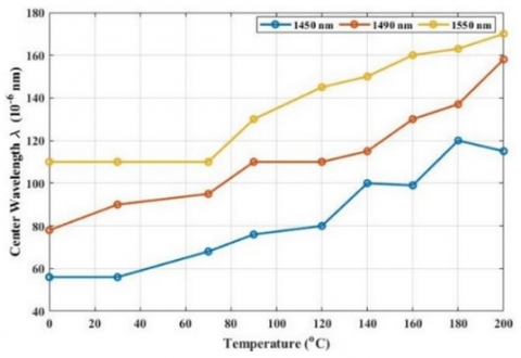
In most cases, the wavelength of these laser diodes is influenced by the injected current and temperature changes. Energy conversion to heat or variations in ambient temperature may cause these temperature fluctuations. This heating leads to instability in the laser's intensity, phase, and wavelength, as shown in Figure 1. As a result, the diode becomes unsuitable for certain applications. The wavelength can vary by 0.1–0.5 nm per 1℃, necessitating temperature control for stability [3, 4].
Effective temperature control is crucial for maintaining a laser diode's constant wavelength. Common methods including those developed by Lehmann et al. [5] and Schulz et al. [6] for temperature control have employed passive or active heat sinks to address this challenge. Lehmann et al. [5]'s approach offered an affordable temperature controller which achieving an accuracy of 0.5℃. This level of precision does not meet the requirements for the interferometer. Conversely, Schulz et al. [6] focused on a high-precision controller with an accuracy of 0.001 at 30℃, but this came with increased costs due to the use of specially designed thermoelectric coolers. The excessive cost and limited range are the main obstacles preventing the use of these approaches in the system.
Figure 1. The effects of temperature on center wavelength [4]
This paper proposes a novel temperature control system designed to overcome the limitations of these previous methods. The primary objectives of this design are to prioritize simplicity, cost-effectiveness, fast response, and ability to effectively tackle temperature-related concerns linked to the fiber-optic interferometer. This work aims to develop a user-friendly laser diode temperature controller with minimal effort. Our works are different from the approaches of Lehmann et al. [5] and Schulz et al. [6] by incorporating cost-effective components for regulating the temperature of the laser diode. The key challenge is to maintain the laser diode's temperature with a standard deviation below 0.1℃. This precise temperature control is crucial for consistent wavelength stabilization and enhances the system's precision and stability. The key contributions of this paper are outlined as follows:
By addressing the specific temperature control issues associated with fiber-optic interferometer systems, our study aims to present a solution. This solution is not only technically advanced but also cost-effective and simpler compared to existing methods.
The remainder of the paper is organized as follows: Section 2 explains fibre optical interferometer system. Section 3 describes the technical temperature controller requirements and constraints. Section 4 describes the architecture of the laser diode temperature controller. Section 5 explains the hardware and software setup and evaluates them. Also, the advantages of our temperature controller are quantified using experimental results in this section. Finally, Section 6 concludes the work.
The interferometer has been widely investigated in scientific and industrial fields for the measurement of small displacements, refractive index changes, and surface irregularities. A Laser interferometry system employs a highly stabilized light source and precise optics to measure distances with great accuracy. The system accuracy depends on environmental stability (such as temperature, air pressure, noises and humidity). Regular calibration using known standards is necessary to maintain precision over time. Repeatability measurements are needed to understand the behavior of the oscillating sensor. These involved recording multiple signals as the optical probe oscillated at a fixed distance from the object being measured [6].
These factors are essential for the system's high precision. Employing interferometric principles, these devices enable micro- or nanometer-scale surface analysis. They operate by splitting the source light into two paths using a beam splitter, which involves a reference and an object surface. These systems can function through either linear or sinusoidal phase shifting methods [1, 2]. The fundamental principle of a laser interferometry system is its ability to detect and measure the changes in phase of the laser light waves. These waves are analyzed for phase differences between the emitted and returning waves after the wave reflected off an object and returned. This difference correlates directly with the distance traveled by the light, enabling precise distance measurements.
In general, the key components of a fibre optical interferometer system work simultaneously for precise object measurement. The laser diode emits a coherent and stable light beam and the beam divides by a splitter into two beams. one is guided using Mirrors/Reflectors towards the measurement object and another to a reference path. these beams. Finally, the detector captures the returning beams and measures the interference pattern formed by the overlapping of the reference and measurement beams. Each component plays a critical role in maintaining the system's accuracy.
The fibre optical interferometer system is constructed from fibre-, micro-optical and electronic components and the important part in the system is called fibre-coupled interferometric sensor [1, 2]. The fibre-coupled interferometric sensor or the whole part for holding the sensor is called micro-optical probe holder, which is, constructed as follows [5, 6].
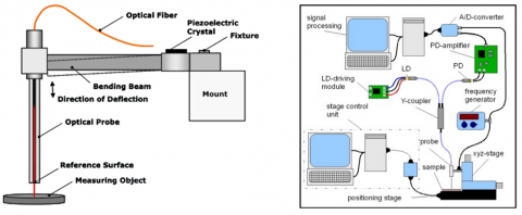
Figure 2. Schematic of (a) micro-optical probe [1] and (b) the fibre optical interferometer [7]
• The micro-optical probe is mounted on a bending beam which is driven by a piezoelectrical actuator, and the bending beam is mounted on an xyz-stage but in this work x and y axes are fixed and the probe can only be moved in z-direction as shown in Figure 2(a).
• The micro-optical probe head is connected to a single mode fiber which splits through Y-coupler to connect the laser diode (DFB laser 1310nm) on one side and a photodiode (PD) on the other side as shown Figure 2(b).
• The piezoelectrical actuator (crystal) is mounted in a frame which is a part of a bending beam. The actuator appears partly above the middle bending beam to bend micro-optical probe when it is expanded by applying a voltage. This actuator is worked to modulate or change the distance between the head probe surface and measuring object. The distance modulation occurs through periodically expanding and contracting of the actuator when a voltage signal such as a sinusoidal signal is applied. This modulation is a mechanical modulation which is called optical path length modulation (OPL) as shown in Figure 2(a).
The optical path difference (OPD) is the difference in the traveling paths of the two beams (the reference beam and the reflected beam from the measured object). Because the head probe oscillates, this OPD will change periodically between constructive and destructive interference, and therefore it modulates the interference signal. The OPL modulation of these partially sinusoidal interference is generated. A height change happening additionally to the OPL modulation causes a phase shift in this basic interference signal that can be precisely evaluated by proper data analysis [1, 2, 7, 8]. The OPL modulation is generated by applying a sinusoidal voltage to the piezoelectric crystal, as mentioned before, which modulates the distance between the object and the reference plane. The mathematical equation of the OPL modulation is expressed by the phase-modulated voltage signal:
$V(t)=V_o \cos \left(\frac{4 \pi}{\lambda}\left\{\tilde{z} \sin \left(2 \pi f_o t\right)+z(t)\right\}\right)$ (1)
where, $V_0$ is the amplitude of the photodiode voltage. $\tilde{z}$ is the maximum changed height of actuator, $z(t)$ is the height of the surface changed with time.
The design of a laser diode temperature controller (LDTC) encompasses two phases: hardware and software. In the hardware phase, components such as a heat sink, temperature sensor, thermoelectric cooler (TEC), housing box, PWM driver, bridge circuit, amplifier, and microcontroller are selected and integrated following detailed calculations. The software phase involves configuring the PID controller and other operational programs. Subsequent subsections will detail the design specifications of the LDTC, focusing on stabilizing the laser diode's temperature to maintain wavelength consistency. Key user-centric features of an effective LDTC include cost-effectiveness, simplicity, low power consumption, high accuracy, reliability, sensitivity, strong wavelength stability, and a temperature controller resolution of ≤ 0.1℃.
3.1 Heat sink
The characteristics of the heat sink, essential for dissipating heat from the laser diode to the ambient air, are integral to the combined function of the heat sink and Thermoelectric Cooler (TEC) in temperature regulation. The selection of an appropriate heat sink is interdependent with the specification of the TEC. This determination utilizes Fourier’s Law, which governs heat conduction. Specifically, in the context of one-dimensional steady-state conduction through a homogenous body, Fourier’s Law simplifies to this principle:
$q=\frac{K A \Delta T}{H}$ (1)
where, $q$ is the heat flow (total heat-transfer rate) Watt, $K$ is the thermal conductivity $\mathrm{Watt} /\left(\mathrm{m}{ }^{\circ} \mathrm{C}\right), A$ is the area normal to the direction of heat flow $\mathrm{m}^2, \Delta T$ is the temperature difference (across height $H)^{\circ} \mathrm{C}, H$ is the height in direction of heat flow.
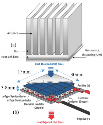
Figure 3. Structure of (a) Heat sink which tradeoffs between number of fine fins and spacing between fins, and (b)TEC element constructs of p and n elements is connected in series which transfers the temperature from code side (object) to hot side (heatsink) [9]
To enhance heat sink design and selection while minimizing material and manufacturing costs, several key factors must be considered [10-13]:
1. A balance between fin density and size is crucial for effective heat dissipation, as depicted in Figure 3(a). Heat sinks with specific fin shapes/profiles are more efficient in heat dissipation.
2. Optimal thermal resistance reduction and conductivity enhancement require perfect contact between the heat sink and the heat source, achieved through various mounting methods and ensuring smooth surfaces.
3. The choice of heat sink material, such as gold, silver, copper, or aluminum, is influenced by their electrical and thermal conductivities and associated costs.
4. Heat sinks with profiled fins are notably more effective in heat dissipation.
5. Effective air circulation through fine fins can be facilitated by a powerful fan, as shown in Figure 3(a).
6. For low-wattage applications, a large aluminum block suffices, but higher wattage demands adherence to the aforementioned requirements.
The heat sink employed in this work is passive and profile in nature, with characteristics such as tall and broad fins, large spaces between fins, and a thick base. Since the use of a fan would introduce unwanted noise into the fibre-optic interferometer setup, we have opted against employing such a method.
3.2 Aluminum mounting box
The aluminum box, a critical component in our design, serves to contact and mount a laser diode to a TEC Peltier (cold side). In the design of the Aluminum Mounting Box, particular attention was given to its dimensions and functionality to ensure optimal performance. The box is precisely crafted with dimensions of 30mm in length, 30mm in breadth, and 10mm in height. To accommodate the essential components, the box is drilled with two specific holes: one with a smooth inner surface, with a diameter of 6.35mm to house the laser diode and closer to the Peltier cooler (cold side), and another with a diameter of 1.8mm for the temperature sensor, as depicted in Figure 4. The temperature sensor hole also extends to a depth of 20mm. These dimensions and adaptations were meticulously calculated to ensure a snug and effective fit for both the laser diode and the temperature sensor, thereby optimizing the thermal management and overall performance of the system.
Plastic screws secure the box to the TEC, enabling adjustable compressive stress while minimizing heat transfer from the heat sink. This approach stabilizes temperature, ensuring laser diode reliability and reducing mounting and maintenance costs compared to thermal glue.
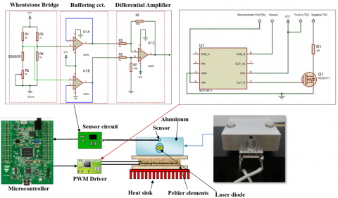
Figure 4. The proposed architecture of a laser temperature controller system
The thermoelectric cooler (TEC) is a solid-state heat pump that uses the Peltier effect to transfer heat from one side (the cold side) to the other (the hot side) through dissimilar semiconductors when direct current (DC) power is applied. Figure 3(b) shows the structure of a thermoelectric cooler. The requirements for choosing TEC are explained as follows [14-18]:
3.4 Temperature sensor
In temperature control systems, temperature sensors are crucial for measuring and safeguarding against temperature-induced distortions. Common types include thermocouples, resistive temperature devices (RTDs), thermistors, and integrated silicon sensors. Selection criteria encompass accuracy, temperature range, response speed, thermal coupling, environmental factors, and cost. In defining sensor requirements for a standard laser cooling system, the selection of an appropriate sensor necessitates the following considerations [19-21]:
Given the specified criteria, the RTD Pt1000, a platinum-chip temperature sensor, is employed due to its advantages including long-term stability in air, reduced noise sensitivity with current excitation, and the ability to generate voltage output with minimal current (<1 mA). This sensor is characterized by its robustness, compactness, linearity, and high sensitivity (±0.01℃).
3.5 Signal conditioning circuits
This section describes the enhancement of transducer outputs into suitable signals for digital conversion, further processing, control, or display. It specifically employs a bridge circuit, notably the Wheatstone bridge, to measure temperature-induced resistance changes in an RTD sensor. Bridges are effective for detecting slight resistance variations. The Wheatstone bridge, sensitive to minor electrical resistance shifts, particularly in temperature, is commonly used. Figure 4 shows a standard Wheatstone bridge configuration with four resistors, powered by voltage or current. The bridge includes ratio arms (resistances R1 and R2), a standard arm (known resistance R3), and an unknown resistance R4. A DC power source connects between points C and D, with points A and B used for balancing [22, 23]. In a balanced Wheatstone bridge, where the ratio of resistances R1 to R4 equals that of R2 to R3, the output voltage measures 0V, as depicted in Figure 4. Criteria for selecting and designing the Wheatstone Bridge include:
This study focuses on the use of differential amplifiers in signal conditioning circuits, primarily for amplification purposes. Amplification is critical for two main reasons: firstly, it enhances signal measurement resolution, which is contingent on the A/D converter's bit count and the ADC's maximum analog input voltage range. Secondly, it improves the signal-to-noise ratio (SNR), a function of the amplifiers' noise rejection capabilities and resistor precision. Additionally, as recorded voltage levels decrease, system vulnerability to noise escalates, necessitating increased gain in the conditioning circuits.
The differential amplifier, essentially an operational amplifier subtractor, facilitates the subtraction of two voltages while rejecting common mode signals. Ideally, its common mode gain (Gcm) is zero, but practically, it is minimal, influenced by the operational amplifier and the matching of external resistors. The effectiveness of an operational amplifier in discarding unwanted signals is best assessed by the differential to common mode gain ratio. The basic configuration of a differential amplifier, as depicted in Figure 4, though rudimentary, is quite effective. However, its limitations include low and unequal impedances at the inverting and non-inverting inputs, adversely affecting the circuit's common-mode rejection ratio (CMRR). Enhancements, such as incorporating high input impedance buffers, are made to this simple design to provide matched high-impedance inputs, thereby minimizing the impact of input source impedances on the circuit's CMRR.
3.6 Thermoelectric cooler driver
A thermoelectric cooler (TEC), specifically the TEC QC 35-1.4-6.0 M, is a solid-state, current-controlled device that produces a heat flux dependent on the current, voltage, and operational duration. We chose the TEC QC 35-1.4-6.0 M for its efficiency and suitability for our system, despite its polarity reversal susceptibility. This model is particularly susceptible to polarity reversal, leading to rapid heating and potential damage within one second, necessitating careful polarity management. The driving criteria for the TEC are outlined in this study [17, 21, 24]:
3.7 Microcontroller and programming software
A microcontroller, tasked with controlling external devices, operates on digital data converted from electrical signals via an ADC. Selection criteria for microcontrollers include:
This study utilizes the STM32F407 microcontroller, equipped with three 12-bit ADC converters and a conversion rate of 1 MHz. The ADC, powered independently between 3.3 and 5.0 volts, allows internal or external reference connections and programmable conversion times across eight discrete ranges (1.5 to 239.5 cycles) [25]. It features 18 multiplexed channels, including 16 for external signals, one linked to an internal temperature sensor, and another to a reference voltage. We chose the STM32F407 microcontroller for the LDTC for its fast processing and ample memory, essential for real-time monitoring and complex algorithms. Its ADC operates in DMA mode, enabling efficient data handling without MCU intervention. Coupled with extensive I/O capabilities, these features ensure precise temperature control and system reliability, meeting the LDTC's specific needs for laser diode stabilization. Various C/C++ integrated development environments (IDEs) are available for efficient software development; however, this research exclusively employs the German SiSy environment, tailored for ARM microcontroller programming in embedded system design, offering extensive support and resources.
3.8 Control system
Control systems are essential due to the complexity or absence of plant models in the design process. PID (Proportional-Integral-Derivative) controllers, effective for nearly linear plants, are prevalent in industry, solving 95% of control problems, with many systems primarily using PI control. These controllers, often integrated with logic and function blocks, manage complex automation tasks in heating, cooling, fluid level, flow, and pressure control. Modern PID controllers, typically microprocessor-based, feature automatic tuning, gain scheduling, and continuous adaptation. The Operational guidelines for PID controllers can be summarized as follows [26, 27]:
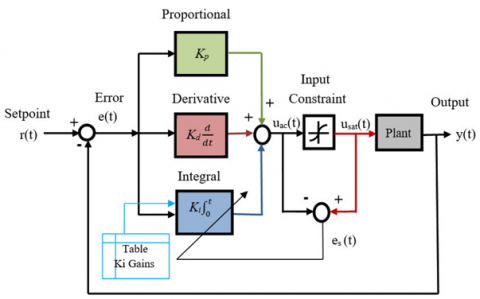
Figure 5. Block diagram of proposed Ziegler-Nichols tuning PID integrated by anti-windup
Figure 5 depicts the PID’s overall structure. The three constants Kp, Ki, and Kd, also known as the proportional, integral, and derivative gains, are the PID design parameters. The PID controller permits inputs from the present, the past, and the future. The optimum equation for a digital PID controller is as follows:
$u(t)=K_p(t) e(t)+K_i(t) T_s(t) \sum_{k=0}^t e_k+K_d \frac{e(t)-e(t-1)}{T_s}$ (3)
where, e(t) is the error of the system response in the t instant; e = ysp-y, y is the measured process variable, Ts is the signal sampling period, and u is the control signal (PWM). The reference variable ysp is often called the set point.
This study focuses on developing a laser diode temperature controller for a fiber-optic interferometer, aiming to create an affordable and reliable temperature regulation system for a laser diode. The laser diode temperature controller is composed of four principal elements: an optical unit (including a DFB laser diode and a fiber-optic interferometer), a thermoelectric cooler (TEC) based transduction and mechanical unit with a heat sink, RTD sensor, and laser diode housing for temperature control, a signal conditioning and TEC driver unit, and a control and processing unit. This last unit employs an STM32F407 microcontroller with a Cortex-M4 core for control signal generation, analog-to-digital conversion, and PID algorithm-based temperature data processing. Figure 4 in our documentation details the system's hardware layout, specifically showing how the heat sink connects to the TEC and aluminum box, and illustrating the integration of sensor and circuit with the microcontroller.
In this study, a 5V power supply is utilized for the entire system, with the TEC's selection influenced by the laser diode's type (InGaAsP DFB laser, PL13N0021FAA-0-0-01) and power constraints. This diode, emitting at a central wavelength of 1310 nm, has a maximum output of 2 mW and operates at a maximum current of 150 mA for the laser and 0.8 mA for the photodiode. Given its low dissipated power (approximately 26 mW), the TEC QC 35-1.4-6.0 M is chosen for efficient cooling, operating below 40% of its maximum voltage and current. The TEC's current and voltage are constrained by a 1Ω resistance and 25 watts power.
We selected the TEC QC 35-1.4-6.0 M for its optimal balance of cooling efficiency, power use, and size, excelling in rapid temperature adjustment and stability, crucial for our precise temperature control needs. Its design, featuring low-height and/or larger cross-section pellets, offers a higher cooling capacity compared to other modules, aligning with the specific cooling capacity requirements of our system.
For temperature sensing, the RTD Pt1000 is selected for its high accuracy, linearity, and simple integration into circuits like the Wheatstone bridge, despite its slower response compared to thermistors. This choice considers factors such as accuracy, response time, temperature range, environmental suitability, ease of use, and cost. The sensor's resistivity demonstrates a linear increase with temperature, as described by the following formula:
$R_T=R_o(1+\alpha T)$ (4)
where, $R$ is the resistance of the sensor at $T, R_o$ is the absolute resistance $1000 \Omega$ of the sensor at $T=0^{\circ} \mathrm{C}$, and $\alpha$ is the RTD sensor temperature coefficient $3.85 \times 10^{-30} \mathrm{C}^{-1}$ between 0 and $100^{\circ} \mathrm{C}$. The RTD sensor temperature coefficient is small, the operating current is recommended to be $0.1 \mathrm{~mA}$ and the maximum current is $1 \mathrm{~mA}$. If the sensor is operated with the maximum current, this causes the sensor to self-heating $\Delta t$ which is expressed as
$\Delta t=I^2 R E$ (5)
In air, the self-heating coefficient (E) is 0.2 °C/mW. At a current of 0.1 mA, self-heating is minimal, but it becomes significant at 1 mA. The chosen operating current for the sensor in this study is 0.5 mA, resulting in a self-heating temperature of approximately 10 µ°C.
Upon selecting the sensor, laser diode, and thermoelectric cooler (TEC), the TEC's geometrical compatibility is dictated by its need for direct physical contact with the laser diode. Optimal contact is achieved through a custom-designed aluminum housing (Al-box) for the laser diode, tailored to minimize thermal resistance between the TEC and the diode. This Al-box, matching the TEC's length (~30 mm), incorporates a 6.35mm diameter hole for the laser diode and a 1.8mm, 20mm long hole for the temperature sensor. The design ensures the RTD sensor fits snugly in the smaller hole, while the larger hole fully encompasses the laser diode. Attachment of the box to the TEC is facilitated by plastic screws, which regulate compressive stress on the TEC and prevent heat transfer from the heat sink to the box via the screws, thereby maintaining diode temperature stability. This screw-based method offers a cost-effective alternative to thermal glue for mounting and part replacement, as illustrated in Figure 4.
The power of the laser diode PL13N0021FAA-0-0-01 is calculated by multiplying the DC applied voltage and current, depending on the datasheet, as shown below. A laser diode's dissipated power is $P=I \times V-P_{\text {out }}=150 \times 10^{-3} \times 1.5-2 \times$ $10^{-3}=0.223$ watt. The laser diode is cooled using a TEC QC $35-1.4-6.0 \mathrm{M}$, whose resistance is determined to be $0.6 \Omega$ when coupled serially with a measured resistance of $1.2 \Omega$ and with the MOSFET switch transistor. Using a 5 -volt power supply and an expected MOSFET voltage of 0.25 volts, we can calculate its current as follows:
$I=\frac{V_{\text {Supply }}-V_{\text {MOSFET }}}{\text { sum of resistances }}=\frac{5-0.25}{0.6+1.2}=2.6389$ $A$
$V_{T E C}=V_{\text {Supply }}-V_{\text {MOSFET }}-V_{\text {Resistance }}=5-0.25-I \times 1.2=1.58332$ $volt$
$P_{T E C}=\frac{V * I}{2}=\frac{2.638 \times 1.58332}{2}=2.177$ $watt$
The total power $P_{\text {tot }}=P_{T E C}+P_{\text {laser }}=2.323$ watt The temperature of hot side $T_h$ is calculated as $T_h=T_{\text {room }}+R_{t h} \times$ $P_{\text {tot }}$, where $T_{\text {room }}$ is the temperature of room $25^{\circ} \mathrm{C}, R_{\text {th }}$ is the thermal resistance $\left({ }^{\circ} \mathrm{C} /\right.$ watt $)$. Assumed temperature of cold side is $10^{\circ} \mathrm{C}$, assumed $R_{\text {th }}$ laser $=0.1^{\circ} \mathrm{C} /$ watt, and $R_{\text {th box }}$ $=0.1^{\circ} \mathrm{C} /$ watt. The thermal resistance of TEC is found by using curves in the datasheet with the intersection of the operating current and voltage, or power. Thermal impedance represents the resistance to the transfer of thermal energy; therefore, lower numerical thermal impedance ratings mean more efficient heat transfer. The temperature change is calculated $\Delta T=T_{\text {hot }}-T_{\text {cold }}=46^{\circ} \mathrm{C}$, from the curve $T_{\text {hot }}=56^{\circ} \mathrm{C}$ and $R_{\text {thTEC }}$ $=\Delta T / Q_{T E C}=462.177=21.13^{\circ} \mathrm{C}$ watt . The thermal resistance $R_{B O X-T E C}$ presents between the box and TEC can be calculated as $R_{B O x-T E C}=0.1+0.1+21.13=21.313^{\circ} \mathrm{C}$ watt. The hot side temperature without heat sink is $T_h=21+21.313 \times 2.323=$ $70.51^{\circ} \mathrm{C}$. The area of the heat sink is calculated by using the equation below as:
$Q_{e q}=k A \Delta T$ (6)
where, $\mathrm{k}$ is the thermal conductivity for Aluminum, $5 \mathrm{~W} / \mathrm{m}^2 \rho^{\circ} \mathrm{C}$, $Q_{e q}$ is the total power of the laser and the TEC. Then $\Delta T$ $=T_{\text {hot }(T E C)}-T_{\text {room }}=70.51-21=49.51^{\circ} \mathrm{C}$ and the cross section of heatsink $A=Q_{e q} k \Delta T=2.323 / 5 \times 49.51=0.009384 \mathrm{~m}^2$ $=93.84 \mathrm{~cm}^2$. The selection of an appropriate heat sink surface area is crucial for maintaining the desired operating temperature of the laser diode. For this purpose, a heat sink with a surface area exceeding $93.84 \mathrm{~cm}^2$ is recommended. In this study, a heat sink with a surface area of $160 \mathrm{~cm}^2$, measuring $16 \mathrm{~cm}$ in length and $10 \mathrm{~cm}$ in width, was utilized.
The subsequent section details a signal conditioning unit comprising a Wheatstone bridge and differential amplifier (forward part) and a PWM driver (feedback part) for TEC operation. Circuit limitations include a 0.5 mA current from the RTD sensor. Resistances R1, R2, and R3 are set at 5kΩ (±0.1%), with a 4kΩ variable resistance Rx linked to the RTD sensor (RRTD=1KΩ at 0°C). This variable resistance defines the maximum desired temperature point (Max-DTP), set at 26°C, influencing the amplifier's gain and the ADC's maximum voltage level. The ADC on the STM microcontroller has a maximum voltage of 3.3 volts, with calculations proceeding in reverse order.
The temperature range (0–26 °C) enables determination of variable resistance, enhancing sensor accuracy due to reduced Max-DTP. However, the microcontroller STM's ADC range (0 to 3.3 volts) limits temperature controller performance. To mitigate the issue of low differential voltage Vba, a buffered differential amplifier with high impedance and effective CMRR is used, powered by a +5V DC source. The LM324 operational amplifier is chosen for its functional benefits and cost-efficiency, ensuring the amplified output is digitally compatible. This design differs from typical differential circuits by using buffers for isolation from the Wheatstone bridge, achieving high impedance and less non-linearity, thus reducing signal distortion. The amplifier, comprising three operational amplifiers, offers a gain of 100 (see Figure 4). Calculations were performed to derive a formula for converting RTD sensor voltage changes into temperature readings for microcontroller use, as follows:
$T=\frac{2 R}{\alpha R_o} \frac{1}{\left(\frac{V_{c c}}{2 V_{b a}}-1\right)}$ (7)
where, $R$ is a resistance $=R 1=R 2=R 3=R 4+R_{\text {sensor }}, R_{\text {sensor }}$ $=R_o+\Delta R, \Delta R$ is the sensor resistance change which is $\Delta R=$ $\alpha \Delta T R_o, R_o$ is the absolute resistance $1000 \Omega$ of the sensor at $\mathrm{T}$ $=0^{\circ} \mathrm{C}$, and $\alpha$ is the RTD sensor temperature coefficient $3.85 \times$ $10^{-3}{ }^{\circ} \mathrm{C}^{-1}$ between 0 and $100^{\circ} \mathrm{C}$, and $V c c$ is a voltage supply. The difference voltage $\left(V_{b a}\right)$ is a voltage between two branches of the Wheatstone bridge as shown in Figure 4. The ADC converts the amplified difference voltage $V_{b a}$ to the integer value of $\mathrm{ADC}$ voltage level $V_{A D C}$ which depends on the resolution of $\mathrm{ADC}\left(2^{\mathrm{No} \text {. of bits }}=2^{12}\right)$.
Thermoelectric coolers (TECs) are controlled via a PWM signal with a $10 \%-90 \%$ adjustable duty cycle, functioning as an on-off switch for cooling and heating operations. A microcontroller generates a low-current PWM, insufficient for the high-current needs of the TEC. Consequently, a MOSFET driver, specifically the MCP14E11, is employed to amplify the current. This driver, capable of delivering a 3 A peak current, operates on a $5 \mathrm{~V}$ supply and requires minimal input current (1 $\mathrm{mA}$ active, $300 \mu \mathrm{A}$ inactive), aligning with the microcontroller's output capacity. The circuit utilizes an IRLR3717 MOSFET transistor to drive the TEC QC 35-1.46.0M with a high-current PWM of approximately $3 \mathrm{~A}$ through a $1 \Omega / 25$ watt resistance. The MCP14E11 driver thus converts the microcontroller's low-power PWM to a high-power signal, as depicted in the circuit diagram (Figure 4), powered externally at 5 volts and $4.5 \mathrm{~A}$.
In this study, the SiSy software is employed for developing C language applications to configure the STM32F407 microcontroller, operating at 168 MHz with 32-bit floating-point capability and a 3.3-volt power supply. Current consumption varies from 50 mA (without peripherals) to 100 mA (with peripherals), depending on clock speed and peripheral usage. GPIO port C is used for configuring pins, with pin 5 designated for ADC1's analog input and pin 6 for PWM signal output in alternate function mode. The ADC, providing temperature data for computer analysis, interfaces via Port B as a serial port, with USART1's transmitter and receiver on pins 6 and 7, supporting up to 84 MHz I/O speed. ADC1 features a 0-3.3volt range, 1 µsec conversion time, and 1 kHz sampling frequency. PWM output is set at a low 1 kHz frequency to avoid resistance heating. Timers TIM1, TIM2, TIM3, TIM4, TIM5, or TIM8 can trigger ADCs and generate PWM outputs, with the timers also managing interrupts for ADC and PWM in this configuration. The overall functioning of digital and software system components starts when an analog signal enters the ADC and continues until PWM is generated. The following steps describe all the microcontroller’s internal operations. The operational procedures are as follows:
This study presents a nonlinear laser temperature control system enhanced by a PID controller. The PID controller, devoid of traditional PID elements, effectively manages nonlinear systems. It integrates three components: proportional, integral, and derivative, based on the error signal, which is the difference between actual and desired temperatures. Optimal temperature regulation is achieved by automatically adjusting PID gains using the Ziegler and Nichols method, with integral term gains modified via a gain table to suit varying temperature setpoints, enhancing stability and performance. This PID system, programmed in C on an STM32F407 ARM microcontroller using SiSy software, processes inputs like actual and target temperatures and outputs a duty cycle for PWM signal generation. The PID operates synchronously with the sampling period, facilitated by timer 2, and its tuning algorithm is detailed in Figure 5. Upon integrating the optical and physical components, the RTD sensor and TEC are linked to the signal conditioning and TEC driver unit. The TEC's anode and cathode connect to the positive power supply and one side of a $1 \Omega / 25$ watts resistor, respectively. The signal conditioning unit comprises solely a differential amplifier, whose output feeds into the analogueto-digital converter of the STM32F4 microcontroller.
The TEC driver includes the MOSFET IRLU3717 and the MCP14E11 transistor driver, with the MOSFET's drain pin attached to the resistor's other side and its gate pin to the transistor driver's output. The transistor driver receives input from the microcontroller's PWM pin. This microcontroller reads the temperature-corresponding voltage from the differential amplifier and generates a low-power PWM signal to operate the transistor driver circuit. The complete setup is detailed in Figure 6.
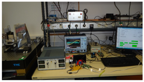
Figure 6. Test the connection of the fibre optical interferometer system and laser diode temperature controller inside the laboratory
The system's performance, including individual components and overall functionality, was assessed through a series of experiments and tests. These evaluations were crucial for verifying assumptions, optimizing operational parameters, and ensuring compliance with specifications. The testing process involved detailed experimental analysis and individual assessment of each component within the cooling system. The evaluation of the optical and physical units involved several tests, summarized as follows:
In the initial experimental test, the laser diode cooling system's robustness and the PID algorithm were evaluated without the optical unit. The testing procedure involved setting a desired temperature in the program, optimizing proportional and derivative gains, tuning the integral gain to reduce steady state error and overshoot while damping oscillations, and documenting the optimal integral gain in the program. This process was repeated across a temperature range of 0 to 26℃.
Ziegler-Nichols tuning PID algorithm integrated by anti-windup is as follows:
Table 1. Controller test parameters without the laser diode
|
Desired Temp. (oC) |
Averaged Temp. (oC) |
Steady State Error (oC) |
Fluctuation (oC) |
|
10 |
10.3561 |
-0.3561 |
0.1006 |
|
11 |
11.0396 |
-0.0396 |
0.0742 |
|
12 |
12.0087 |
-0.0087 |
0.0722 |
|
13 |
12.9899 |
0.0101 |
0.0730 |
|
14 |
13.9776 |
0.0224 |
0.0630 |
|
15 |
14.9529 |
0.0471 |
0.0653 |
|
16 |
15.9406 |
0.0594 |
0.0543 |
|
17 |
16.9423 |
0.0577 |
0.0667 |
|
18 |
17.9600 |
0.0400 |
0.0325 |
|
19 |
18.9456 |
0.0544 |
0.0256 |
|
20 |
19.8995 |
0.1005 |
0.0532 |
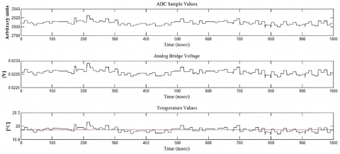
In our study, the temperature control system was designed for a wide 0 to 26°C range, but testing focused on the 10 to 20°C range, aligning with the laser diode's optimal operating temperatures. This approach ensured thorough evaluation of the system's performance under conditions most critical for the diode's functionality. Tests using a yellow hot lamp and human body temperature demonstrated the system's rapid response in returning to setpoints, attributed to the effective integral PID gain. This gain minimizes the overshoot, dampens oscillations below 0.1°C, and maintains a low steady-state error. Figure 7 illustrates these tests at 20°C, presenting data on ADC sampling values, voltage difference on the Wheatstone bridge, and the RTD sensor's temperature readings. At 20°C, temperature fluctuations were 0.0256 (standard deviation) and steady-state error was 0.0544 (average temperature deviation from setpoint), with the red line in Figure 7 representing the average temperature. These tests also emphasized the importance of time-dependent temperature stability.
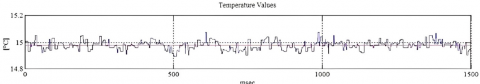
The system's time to reach steady state from room temperature varies between 1-2 minutes, faster than the reverse process. Stability was confirmed over 60 minutes, with fluctuations and steady state errors under 0.1, as detailed in Table 1. The controller's performance was less optimal at a 10℃ range, with a resolution of 0.1 and a steady state error of 0.3561. Figure 8 shows another example of the desired temperature of 16℃ that is read by the controller. Table 1 presents user-selected temperatures and corresponding averaged measured temperatures for error and fluctuation analysis. System testing without a laser diode met all objectives, as shown in Table 1. A DFB laser diode was then tested, placed in the housing box and connected to an interferometer system via optical fiber, with insulated wiring to minimize electromagnetic interference. The interferometer system, using a natural method, indirectly measures wavelength stability of the laser diode. The system setup involves a common path interferometer (Figure 9) and uses a 1310 nm wavelength. Measurements were taken on a plane mirror, averaging height values over 2000 readings, and repeated ten times for reliability, as shown in Table 2. Temperature-induced variations were observed, as demonstrated in Figure 10.
Figure 7. The desired temperature 20℃ reads by controller
Figure 8. The desired temperature 16℃ reads by controller
Figure 9. Sketch of the common path interferometer
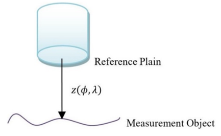
Eq. (8) defines the absolute height $z(\varphi, \lambda)$ relative to the reference plane, addressing the phase ambiguity issue as initially derived in 1 .
$z(\varphi, \lambda)=\frac{\varphi \lambda}{4 \pi}$ (8)
To calculate wavelength change $(\Delta \lambda)$, the absolute height equation is analyzed, and the absolute height measured. Measurement suitability is assessed using the law of propagation of uncertainty, with the general absolute error defined accordingly.
$\Delta y=\frac{\partial y}{\partial x_1} \Delta x_1+\frac{\partial y}{\partial x_2} \Delta x_2+\cdots$ (9)
Applying Eq. (8) under the assumption of a constant phase to Eq. (9) yields the following result:
$\Delta z(\phi, \lambda)=\frac{\phi \Delta \lambda}{4 \pi}$ (10)
The substitution of Eq. (8) into Eq. (10) eliminates the phase, yielding a general equation employed in this study.
$\Delta z(\phi, \lambda)=\frac{\Delta \lambda}{\lambda} z(\phi, \lambda)$ (11)
The altered absolute heights were assessed at two distinct temperatures, T1 and T2, facilitating the estimation of $\Delta \lambda$ and subsequent reorganization of Eq. (11).
$\Delta \lambda=\frac{\lambda_1}{z_{T 1}(\varphi, \lambda)}\left(z_{T 1}\left(\varphi, \lambda_1\right)-z_{T 2}\left(\varphi, \lambda_2\right)\right)$ (12)
Eq. (12) involves the calculation of the change in wavelength $(\Delta \lambda)$ by measuring the height difference $(\Delta z)$ of a micro-optical probe in an interferometer system. At a fixed position called the zero position, the physical height of the micro-optical probe (z) remains constant at $10 \mu \mathrm{m}$ (is assumed as $z T 1(\varphi, \lambda)$ ), assumed to be the same at all temperatures. The interferometer system measures the virtual height between the probe and the object, enabling the determination of the laser diode's wavelength, which is $1310 \mathrm{~nm}$. To calculate the wavelength change, the parameters mentioned above are used in Eq. (12).
$\Delta \lambda=131 \times 10^{-3} \Delta z$ (13)
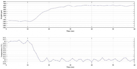
Figure 10. Variations in object measurement corresponding to a 1°C change in temperature
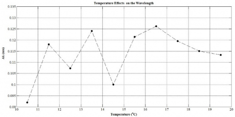
Figure 11. Effects of temperature change 1°C on the wavelength of the laser diode
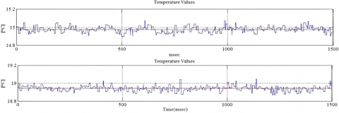
Figure 12. Temperature results from the controller using the DFB laser diode (15℃ and 19℃)
The cooling system's efficacy is evaluated via a laser diode, measuring temperature variations at distinct points. Measurements start at 20℃, decreasing in 1℃ intervals every 10 seconds. Figure 11 shows the temperature's effect on the laser diode’s wavelength, with a maximum and minimum wavelength shift of 0.1262 nm and 0.092 nm. Our results validate a 0.1 nm per ℃ wavelength change in the DBF laser diode, aligning with datasheet specifications. Notably, minimal wavelength variation occurs at 10℃, indicating negligible impact of 1 ℃ change at lower temperatures.
In the final testing phase, the laser diode cooling system's performance is assessed by monitoring temperature changes during operation. Figure 12 presents temperature data from 10℃ to 20℃, processed by Matlab. Table 3 shows the standard deviation and steady-state error, revealing optimal precision at 11℃ (∓0.0013℃), followed by 10℃ (∓0.0042℃). Contrasting with a previous study (6) that used a costlier DFB laser diode with two built-in thermoelectric coolers, our more affordable laser diode, lacking these coolers, yielded surprising and superior results.
The second experiment, utilizing a laser diode, surpasses the initial test due to two key factors: complete enclosure of the laser diode by an aluminum housing and the inherently low power of most DFB laser diodes, as previously discussed.
Table 2. Measurement of object height at a constant temperature of T=22.4℃
|
Height Difference Optical (nm) |
Height Difference Piezo (nm) |
|
94575.4324 |
94913.5325 |
|
94599.7348 |
94910.1466 |
|
94638.8753 |
94905.7947 |
Table 3 Controller test parameters the laser diode
|
Desired Temp. (℃) |
Averaged Temp. (℃) |
Steady State Error (℃) |
Fluctuation (℃) |
|
10 |
9.9958 |
0.0042 |
0.0473 |
|
11 |
10.9987 |
0.0013 |
0.0567 |
|
12 |
11.9765 |
0.0235 |
0.0594 |
|
13 |
12.9890 |
0.0104 |
0.0358 |
|
14 |
13.9891 |
0.0108 |
0.0441 |
|
15 |
14.9779 |
0.0221 |
0.0331 |
|
16 |
15.9719 |
0.0281 |
0.0287 |
|
17 |
16.9633 |
0.0366 |
0.0266 |
|
18 |
17.9641 |
0.0248 |
0.0359 |
|
19 |
18.9713 |
0.0287 |
0.0334 |
This work presents a comprehensive study on the design and implementation of a temperature controller for a laser diode in a fiber-optic interferometer system. The technology’s benefits are primarily its simplicity, cost-effectiveness, fast response, and ability to address specific temperature issues associated with the fiber-optic interferometer. This work aims to develop a user-friendly laser diode temperature controller with minimal effort. It will ensure a consistent temperature for the diode by employing two key principles: cost-effective components and straightforward circuits, and precise temperature measurements. The design of the temperature controller is simple and this simplicity reduces the risk of system overhead and potential noise, which could negatively impact the performance of the interferometer.
This research describes a method for controlling temperature within a program. It encompasses manually setting the target temperature, fine-tuning both the proportional and derivative gains, and adjusting the PID's integral gain to reduce both steady-state error and overshoot. The optimal integral gain is then tabulated. A simple PID controller, used with an integral gains table and adapted gains, mitigates nonlinear behavior and saturation. The system, enclosed in an aluminum box to minimize noise and air impact, employs a low-power DFB laser diode known for high wavelength stability. A variable resistance can adjust the maximum temperature, balanced against the sensor’s temperature resolution. Furthermore, the study established a correlation between the shift in wavelength due to temperature variations and the virtual distance between the probe and the object.
Significantly, the study has demonstrated quantifiable improvements in the performance of the fiber-optic interferometer system through experimental evaluations. The temperature controller consistently maintained the diode temperature, as evidenced by a range of steady-state errors spanning from a low of 0.0087℃ to a high of 0.3561℃, with corresponding temperature resolution improvements. The conducted experiments, performed both with and without the utilization of a laser, substantiated the efficiency of the proposed design. The observed range of steady-state errors spanned from 0.3561℃ at 10℃ (in the worst-case scenario) to 0.0087℃ at 12℃ (in the best-case scenario). Similarly, the temperature resolution varied from 0.1006℃ (worst case) to 0.0331℃ (best case), thereby corroborating the success of the research. The study effectively meets the initial research questions and presents a practical solution to a major challenge in fiber-optic interferometry. The innovative and effective design of the LDTC establishes a new benchmark, leading to more reliable and precise optical measurement systems.
I extend my sincere thanks to the University of Kassel, particularly the Department of Electrical Engineering and Computer Science, Measurement Technology division, for their crucial support in this research. Their resources and guidance were indispensable to the successful completion of this study.
[1] Schulz, M., Lehmann, P. (2013). Measurement of distance changes using a fibre-coupled common-path interferometer with mechanical path length modulation. Measurement Science and Technology, 24(6): 065202. https://doi.org/10.1088/0957-0233/24/6/065202
[2] Schake, M., Schulz, M., Lehmann, P. (2015). High-resolution fiber-coupled interferometric point sensor for micro- and nano-metrology. tm - Technisches Messen, 82(7-8): 367-376. https://doi.org/10.1515/teme-2015-0006
[3] Aho, A.T., Viheriälä, J., Virtanen, H., Uusitalo, T., Guina, M. (2018). High-power 1.5- μm broad area laser diodes wavelength stabilized by surface gratings. IEEE Photonics Technology Letters, 30(21): 21. https://doi.org/10.1109/LPT.2018.2870304
[4] Ab-Rahman, M.S., Shuhaimi, N.I. (2011). The effect of temperature on the performance of uncooled semiconductor laser diode in optical network. Journal of Computer Science, 8(1): 84-88. https://doi.org/10.3844/jcssp.2012.84.88
[5] Lehmann, P., Schulz, M., Niehues, J. (2009). Fiber optic interferometric sensor based on mechanical oscillation. Optical Measurement Systems for Industrial Inspection, 7389: 380-388. https://doi.org/10.1117/12.827510
[6] Schulz, M., Lehmann, P., Niehues, J. (2010). Fiber optical interferometric sensor based on a piezo-driven oscillation. SPIE Optical Engineering + Applications, 7790: 282-292. https://doi.org/10.1117/12.860672
[7] Lehmann, P., Schulz, M. (2011). Fiber-coupled microoptcal interferometric sensor for precision engineering applications. In TC14 LMPMI Symposium 2011, Braunschweig, Germany, pp. 1-12.
[8] Knell, H., Schake, M., Schulz, M., Lehmann, P. (2014). Interferometric sensors based on sinusoidal optical path length modulation. Optical Micro- and Nanometrology V, 9132: 118-127. https://doi.org/10.1117/12.2051508
[9] Hermoelectric/ peltier cooling. Accessed on Jun. 21, 2021. Available: https://www.Thermo.Com.
[10] Lee, S. (1995). Optimum design and selection of heat sinks. IEEE Transactions on Components, Packaging, and Manufacturing Technology: Part A, 18(4): 4. https://doi.org/10.1109/95.477468
[11] Shah, A., Sammakia, B.G., Srihari, H., Ramakrishna, K. (2004). A numerical study of the thermal performance of an impingement heat sink-fin shape optimization. IEEE Transactions on Components and Packaging Technologies, 27(4): 710-717. https://doi.org/10.1109/TCAPT.2004.838879
[12] Cao, J. (2011). Study on three-dimensional numerical simulation of the influence of fin spacing on the power of heat sink and heat dissipation. In 2011 Asia-Pacific Power and Energy Engineering Conference, pp. 1-4. https://doi.org/10.1109/APPEEC.2011.5747704
[13] Xia, G., Zhao, H., Zhang, J., Yang, H., Feng, B., Zhang, Q., Song, X. (2021). Study on performance of the thermoelectric cooling device with novel subchannel finned heat sink. Energies, 15(1): 145. https://doi.org/10.3390/en15010145
[14] Huang, B.J., Chin, C.J., Duang, C.L. (2000). A design method of thermoelectric cooler. International Journal of Refrigeration,23(3):208-218. https://doi.org/10.1016/S0140-7007(99)00046-8
[15] Ibañez-Puy, M., Bermejo-Busto, J., Martín-Gómez, C., Vidaurre-Arbizu, M., Sacristán-Fernández, J.A. (2017). Thermoelectric cooling heating unit performance under real conditions. Applied Energy, 200: 303-314. https://doi.org/10.1016/j.apenergy.2017.05.020
[16] Thermoelectric Coolers Introduction - the Basics. Accessed: Apr. 12, 2023. Available: https://www.tec-microsystems.com/faq/thermoelectric-coolers-intro.html
[17] Pitaloka, D.H., Ikhsani, R.N., Naba, A., Sakti, S.P. (2019). Thermoelectric-based temperature control for rapid heating and cooling. In IOP Conference Series: Materials Science and Engineering, Malang, Indonesia, p.032026.https://doi.org/10.1088/1757-899X/546/3/032026
[18] Siahmargoi, M., Rahbar, N., Kargarsharifabad, H., Sadati, S.E., Asadi, A. (2019). An experimental study on the performance evaluation and thermodynamic modeling of a thermoelectric cooler combined with two heatsinks. Scientific Reports, 9(1): 20336. https://doi.org/10.1038/s41598-019-56672-9
[19] Morris, A.S., Langari, R. (2016). Sensor technologies. In Measurement and Instrumentation (Second Edition), Boston, USA: Academic Press, pp. 375-405.
[20] Lundström, H., Mattsson, M. (2021). Modified thermocouple sensor and external reference junction enhance accuracy in indoor air temperature measurements. Sensors, 21(19): 6577. https://doi.org/10.3390/s21196577
[21] Yüksel, Y. (2010). Thermoelectric cooling of a pulsed mode 1064 nm diode pumped Nd: Yag laser. Master Thesis, Middle East Technical University. Accessed: Apr. 12, 2023. Available: https://open.metu.edu.tr/handle/11511/20185
[22] Park, J., Mackay, S. (2003). Signal conditioning. In J. Park & S. Mackay (Eds.), Practical data acquisition for instrumentation and control systems, Oxford, England: Newnes, pp. 36-66.
[23] Morris, A.S., Langari, R. (2016). Data acquisition and signal processing. In A. S. Morris & R. Langari (Eds.): Measurement and Instrumentation (Second Edition), Boston, USA: Academic Press, pp. 145-175.
[24] Nagy, M.J., Roman, S.J. (1999). The effect of pulse width modulation (PWM) frequency on the reliability of thermoelectric modules. In Eighteenth International Conference on Thermoelectrics. Proceedings, ICT’99 (Cat. No.99TH8407), Baltimore, MD, USA, pp. 123-125. https://doi.org/10.1109/ICT.1999.843348
[25] Ünsalan, C., Gürhan, H.D., Yücel, M.E. (2023). Embedded System Design with ARM Cortex-M Microcontrollers: Applications with C, C++ MicroPython. Springer International Publishing, Germany.
[26] Hasan, S., Ismael, A.M. (2021). Implementable self-learning PID controller using least mean square adaptive algorithm. Iraqi Journal of Science, 148-154. https://doi.org/10.24996/ijs.2021.SI.1.20
[27] Grüne, L. (2019). Dynamic Programming, Optimal Control and Model Predictive Control. In S. V. Raković & W. S. Levine (Eds.): Handbook of Model Predictive Control, Switzerland: Birkhäuser, Cham, pp. 29-52. https://doi.org/10.1007/978-3-319-77489-3_2