Kamel Boukoffa*![]() | Abderrezak Metatla
| Abderrezak Metatla![]() | Ilyes Louahem Msabah
| Ilyes Louahem Msabah![]() | Samia Benzahioul
| Samia Benzahioul
© 2023 IIETA. This article is published by IIETA and is licensed under the CC BY 4.0 license (http://creativecommons.org/licenses/by/4.0/).
OPEN ACCESS
The detection and identification of some types of faults in PV systems is often difficult, because it is not possible to distinguish the noise coming from external factors and the influence of some faults on the parameters generated by PV systems. Until today, scientific works have focused more on the detection and identification of faults affecting a PV system. These works are focused on the application of different sophisticated and unsophisticated techniques. Therefore, the possibility of obtaining significant information about faults requires the development of more advanced techniques. The presented work consists of studying the influence of defects on the behavior of a photovoltaic system. In the first part, the work aims to present a signal processing technique based on the analysis of structured residual. In the first step of this part, the generated currents by the GPV are presented with the three operating modes: healthy, shading fault and progressive resistance fault, in the second step, the prediction errors of the current vectors from the three operating scenarios of the GPV are calculated. The evaluation of the developed approach, shows the efficiency and the identification precision of this method. In the second part, a technique based on the SEA method (Shape exchange algorithm) is presented whose diagnostic indicators were calculated, these indicators were classified according to their degree of criticality into three main categories. The obtained results show the effectiveness of this technique and the possibility of further increasing the detection and identification performance of faults in the PV system.
PV system, fault diagnosis, shading defect, identification, residual analysis, detection, indicators method, sensitivity analysis
In recent years, and thanks to various factors such as the reduction of production costs and supporting policies, the solar energy market has experienced a very considerable growth in the world. Like any physical process, the photovoltaic (PV) system is subjected to different constraints during its operation which lead to a reduction in yield, and so, a drop in the performance of the PV system [1].
Therefore, it is essential to put a clear policy to detect and locate faults in a photovoltaic installation. A study proposed in the study [2], this study is summarized in four steps. In the first step, the authors used a real database to model the photovoltaic installation, it is followed by a stage for introducing healthy and faulty operating scenarios and the analysis of the relative modifications on the I-V characteristic. In the third step, the authors evaluated the effects of faults on significant photovoltaic system parameters. In the last step, a proposed of several fault signature tables was made to evaluate the faults effect in the photovoltaic system. Another study developed in the study [3], the author proposes a diagnostic method based on parameters that can be easily calculated from the I-V characteristic, the application of the fuzzy logic technique allows the evaluation of this diagnostic method. A technique has been developed in the study [4], whose author proposed a method for monitoring and diagnosing faults in real time in photovoltaic systems, this method is based on a comparison between the performances of a defective photovoltaic module with its specific model. The authors [5] have proposed an approach for the detection and analysis of defects based on the vibration ultrasonic waves analysis. A technique proposed in the study [6] based on determining the number of PV modules that are short-circuited or open-circuited in a single PV string. The authors [7] proposed a diagnostic procedure based on the study of parameters variation in particular $\left(I_{m p p}, V_{m p p}, P_{m p p}\right)$.
A new technique proposed in the study [8] for the detection of the number of faulty PV modules, this technique is based on the extension theory. Another approach based on neural network (ANN) proposed in the study [9]. The authors [10] propose a technique based on three tools for the performance of the diagnosis tool. Another approach for the monitoring and diagnosis of some types of faults caused by snowfall, this approach is based on the use of climate data provided by satellite [11]. There are also some diagnosis methods that use very sophisticated procedures such as (infrared thermography) [12]. Another monitoring and diagnostic method proposed in the study [13, 14] based on the evaluation of power losses in the PV generator. The authors [15] presented a technique based on earth capacitance measurement to locate disconnected PV modules. An approach based on the Fourier series was used for the detection of the arc fault and to make the difference between a series or parallel PV module [16]. The authors [17] propose a diagnosis method based on the extension theory for the detection of faulty PV modules in the different groups. Another diagnosis method based on fuzzy logic proposed in study [18]. The authors [19] presented a fault detection algorithm based on robust statistics for locating failed PV modules. There are several algorithms based on the comparison between modeled and measured PV modules for faults identification [6]. An approach based on parametric models and meteorological conditions used for the prediction of the power produced by the PV panel [20]. Several research works propose circuit models for estimating the power produced by PV modules [21-23]. Currently, a new generation of fault diagnosis methods based on the measurement of the partial or total I-V characteristic [24], several research works suggested diagnosis techniques based on the analysis of the I-V characteristic in order to obtain better results [25, 26].
The state of the art has shown that many works have focused only on the effect of the various faults on the extracted power by the PV generator, the results of these works are limited to show the nature of defects that affect the PV system.
The presented work in this paper is divided into two parts. In the first part a new approach for faults diagnosis in PV generators based on the analysis of structured residual is proposed [27], this approach makes it possible to reliably detect and identify the various faults in the PV system. In the second part a new diagnostic technique SEA (Shape exchange algorithm) [28] based on the sensitivity analysis of the diagnostic indicators is proposed, this technique also allowed us to further increase the reliability of the fault detection and identification operation. The validation of the two approaches was carried out on a real database with two completely different types of defects (shading and connection resistance defect), the obtained results are very promising.
A defect in a PV system is any accidental modification which affect their normal operation. These defects that can be occurred during its manufacture, its installation or during its operation, these latter cause a drop in yield and sometimes the total stopping of PV production [29].
This work presents the most two defects affecting the PV system, which are shading and connection resistance fault, the different operating modes of the chosen photovoltaic system are listed in Table 1.
Table 1. Operating mode of the PV generator
|
PVG states |
Number of test |
Causes and effects |
|
Healthy state |
1529 |
Optimal operation of the PV system |
|
Shading defect |
657 |
Causes a low generated voltage and low power |
|
Connection resistance defect |
124 |
Degradation of interconnections, Crack, Corrosion of connections between cells, defects related to the problem of the increase in the connection resistance between two PV modules. |
|
Total |
2310 |
|
In the rest of the work, the following notations are used to designate the different operating scenarios of the PV generator, Healthy state (h), shading fault (S) and connection resistance fault (R).
A test bench was created to realize the different fault scenarios or the operating modes of the PV generator (Table 1). The used photovoltaic system consists of a PV string, a string is made up of three poly- crystalain PV panels (CLS-220P from CHINALIGHT Solar) connected in series, which is characterized by: STC Power Rating Pmp=220(W), Open Circuit Voltage Voc=36.8(V), Short Circuit Current Isc=8.24 (A), Voltage at Maximim Power Vmp=28.9(V), Current at Maximim Power Imp=7.61(A), Panel Efficiency 13.4%, Fill Factor 72.6%, Power Tolerance -1.00% ~ 1.00%, Maximum System Voltage Vmax 1000(V) [2].
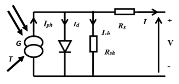
The PV cell model presented in Figure 1 is characterized by five parameters; $I_{p h}(A)$ (photo- generated current).
$R_{\text {sh ohm }}(\mathrm{ohms})$ (shunt resistance), $R_s (ohms)$ (series resistance), $I_0$(A) (saturation current) and a (diode ideality factor), thermal module voltage ($V_{t e}=T \cdot N_s \cdot \frac{k b}{q}(V)$), cell temperature (T), electron charge $q=1.60210^{-19} C$.
Boltzman constant ( $k b=1.38110^{-23} \mathrm{~J} / \mathrm{K}$), solar cell number in series ($N_s$), are known parameters, the relation between current I and voltage V is explained by Eq. (1) [2].
$I=I_{p h}-I_0 \times\left(\exp \left(\frac{V-I \times R_s}{a \times V_{t e}}\right)-1\right)-\frac{V-I \times R_s}{R_{s h}}$ (1)
Figure 1. One diode model of PV cell
In this paper, an approach for detecting and identifying faults in the PV generator is proposed. This approach is carried out in two steps, a fault detection step and another for identification.
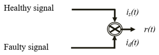
The principle of fault detection is illustrated in the following schema.
Figure 2. Detection principle
In Figure 2, fault detection is based on the calculation of the prediction error between the current supplied by the PV generator in the healthy state and the faulty state, the following mathematical formulation expresses the method.
$r(t)=i_s(t)-i_d(t)$ (2)
where, $r(t)$ is prediction error, $i_s(t)$ and $i_d(t)$; present respectively the Current $I(\mathrm{~A})$ generated by the $\mathrm{PV}$ generator for healthy state and faulty state.
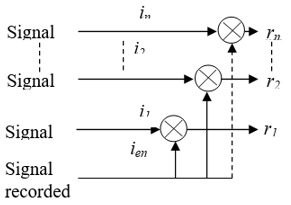
The fault identification method proposed in this context is based on the analysis of the structured residual calculated from the difference between the prediction error of the recorded signal and the errors of the other signals, the schema of identification methodology is shown in Figure 3.
Figure 3. Identification principle
This can be reformulated mathematically by the following algorithm:
$\left\{\begin{aligned} r_1(t) & =i_{e n}(t)-i_1(t) \\ r_2(t) & =i_{e n}(t)-i_2(t) \\ & \cdots \cdots \cdots \cdots \cdots \\ r_n(t) & =i_{e n}(t)-i_n(t)\end{aligned}\right.$ (3)
where, $i_{e n}(t)$; is the recorded current signal.
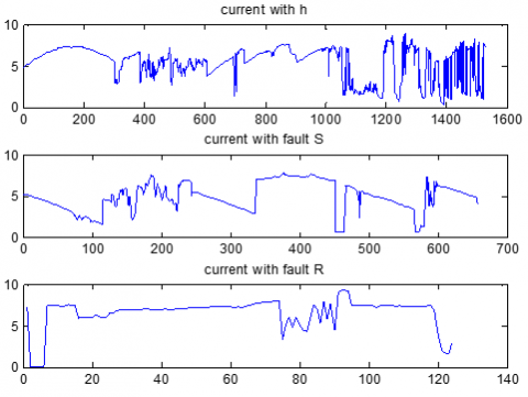
The residual method algorithm is implemented in the MATLAB 2018 environment, Figure 4 shows the currents generated by the PV generator in different operating modes. The first one shows the current in the healthy state with a test number of 1526, the second shows the shading defects with a 657 test number, and the last curve shows the current in the case of connection resistance fault with a test number of 124 (Table 1).
Figure 4. The current generated by the PV generator in a different scenario
The evolution of the three currents, clearly show that the generator operates under different conditions causing disturbances on the current generated by the PV system.
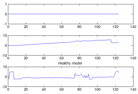
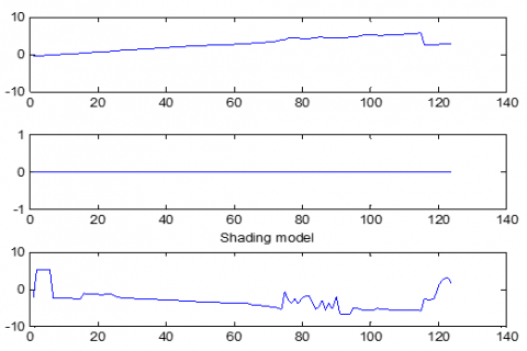
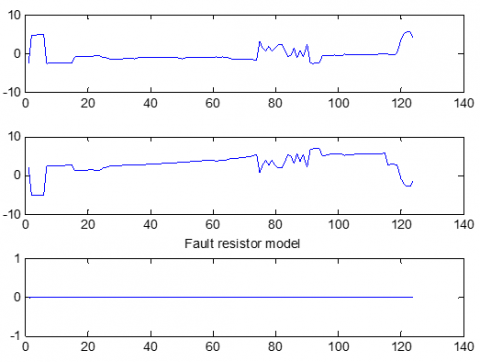
Figures 5, 6 and 7 show the prediction residuals of the three operating modes of the PV generator compared to a recorded operating mode.
Figure 5. Identification residual, case of recorded healthy operation
Figure 6. Identification residual, case of recorded shading fault
Figure 7. Identification residual, case of recorded connection resistance fault
Defect identification is performed offline, based on the analysis of the residual r1, r2 and r3 resulting from the comparison of the residuals obtained with the three operating modes, Figure 5 illustrates the identification residual in the healthy case of the PV system, the residual r1(t) is around 0 while the residuals r2(t) and r3(t) are significantly disturbed. The Figure 6 shows the identification residual in the defect shading case , The residual r2(t) is around 0 while the residuals r1(t) and r3(t) vary significantly, finally Figure 7 shows the residual in the case of connection resistance fault, The residual r3(t) is around 0 while the residuals r1(t) and r2(t) vary significantly. The analysis of the three obtained residuals in each case is sufficient to identify the type of defect. The matrix below further explains the fault identification.
$S=\left(\begin{array}{llll} & h & f_{s h} & f_r \\ r_1 & 0 & 1 & 1 \\ r_2 & 1 & 0 & 1 \\ r_3 & 1 & 1 & 0\end{array}\right)$
So to be able to detect and identify the presence of faults in the PV generator, we often consider the residual in the healthy state as a reference residual, the obtained residuals from the faulty signals lead to a better fault diagnosis. Therefore obtained results are very satisfactory for online detection and offline identification of the two types of faults, shading and connection resistance fault.
To make the detection and identification operation even better, more reliable and efficient, this work proposes the identification residuals in the form of samples, by the use of the autocorrelation function and the partial autocorrelation function in the intervals or confidence limits, which allows us to have the situation of the samples regarding to the confidence intervals for the three operating modes of the PV generator.
Autocorrelation is the linear dependence of a variable on itself at two times. For stationary processes, the autocorrelation between two observations depends only on the time difference, it is defined by:
$\operatorname{Cov}\left(y_t, y_{t-h}\right)=y_h$ (4)
The time difference h of the autocorrelation is given by:
$\rho_h=\operatorname{Corr}\left(y_t-y_{t-h}\right)=\frac{y_h}{y_0}$ (5)
The denominator $y_0$ is the covariance with delay 0, Partial autocorrelation is the autocorrelation between $y_t$ and $y_{t-h}$ after removing any linear dependence on $y_1, y_2, \ldots y_{t-h}+1$.
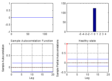
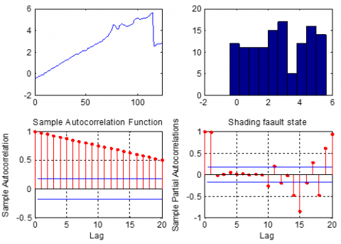
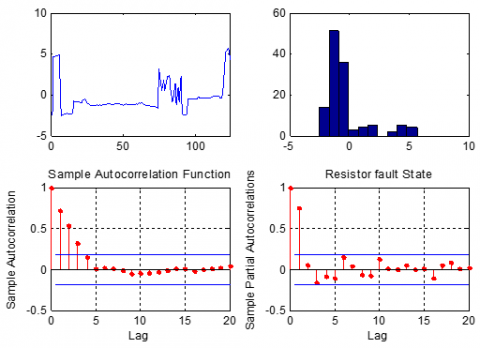
Figures 8, 9 and 10 clearly show the identification residuals with a spectral representation, followed by the autocorrelation and the partial autocorrelation for each sample of the three operating modes of the PV generator.
The obtained results show that, the healthy case contains a single spectrum corresponds to the fundamental with zero delay, the autocorrelation values of the samples lie within the confidence intervals. Therefore, it can be concluded that the residual in this case is a measurement noise (measurement error). In the cases of the tow defects it’s noted that in the fundamental spectrum with different frequency values are found, which corresponds to the effects of faults on the characteristics of the PV generator, but the autocorrelation values clearly exceed the confidence limits of the measurement noise. The PV generator didn’t take into account all the signal, therefore the residual consist of the signal plus the fault.
Figure 8. Identification residual for healthy case; spectrum, autocorrelation, partial autocorrelation of samples
Figure 9. Identification residual for shading; spectrum, autocorrelation, partial autocorrelation of samples
Figure 10. Identification residual for resistance defect; spectrum, autocorrelation, partial autocorrelation of samples
Sensitivity analysis in diagnosis field of photovoltaic systems is very necessary to better understand the influence of faults on the measured I-V characteristic behaviors, in particular the shading fault and connection resistance fault. To perform sensitivity analysis for diagnosis, a new method SEA is applied, this method is based on the analysis of the variation degree of the diagnostic indicators caused by the I-V characteristic deformation in different areas due to the presence of the two defects mentioned above. Therefore the objective of this part of work is to know which parameters are the most sensitive to the appearance of each type of fault compared to the other parameters. The application of the SEA method allowed us to clearly determine among the eleven calculated parameters that which are the most sensitive to the shading fault or to connection resistance fault. We have classified the eleven parameters into three main categories, according to their degrees of criticality (high sensitivity, medium sensitivity and low sensitivity).
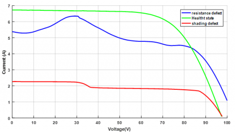
When both shading and resistance faults attack the PV module, they really cause a large deformation in the different areas of the I-V characteristic (Figure 10).
Figure 11. The measured I-V characteristic with and without fault
After the acquisition of the irradiance and the temperature, using electronic load allowed us to measure the current and voltage of the I-V characteristic for the three panels (Figure 11). From the obtained database, it is chosen 105 measurements of the I-V characteristic among 1529 for the healthy state, 105 measurements among 657 for shading defect, 105 measurements among 124 measurements for the resistance fault. The chosen measurements meet the condition $G \geq 500\left(W / m^2\right)$ which is close to the standard test condition Gstc=1000 W/m² et Tstc=25℃.
For each test, the measurement of the irradiance G, the temperature T and the measurement of current I and voltage V are recorded. The diagnostic indicators of Table 2 are calculated using the equations of each indicator, which are shown in Table 2, only six tests are chosen among 105 for just show the extracted diagnostic indicators.
8.1 Equivalent thermal voltage
The equivalent thermal voltage is very sensitive to the appearance of certain types of partial shading which have a major influence on the I-V characteristic, this impact due to the activation of the bypass diode and also the presence of inflection point.
$V_{t e}=\frac{\left(2 V_{m p p}-V_{o c}\right)\left(I_{s c}-I_{m p p}\right)}{I_{m p p}-\left(I_{s c}-I_{m p p}\right) \ln \left(\frac{I_{s c}-I_{m p p}}{I_{s c}}\right)}$ (6)
where, Vmpp (V) is the voltage at the maximum power point Mpp, the Impp is the current at the point Mpp and Vocis the open circuit voltage (V) determined with Isc (A) from the I-V characteristic curve [3].
8.2 Maximum power point factor
There are other types of shading that are uniform, this type of fault does not generate a significant mismatch able to activating the bypass diode and to be detected by the $V_{t e}(V)$ parameter, in this case the Mppf parameter is proposed which calculated based on the irradiance G(w/m2) measured by the installed sensor [3].
$M_{p p f}=\frac{G}{G_{s t c} \cdot I_{m p p}}$ (7)
8.3 Fill factor
This diagnostic indicator is very sensitive to detecting power losses causing the increase of series resistance of the three modules, the power loss is due to the existence of certain types of faults such as shading and connection resistance fault, the FF is also sensitive to the rapid variation of irradiance and temperature [3].
$F F=\frac{I_{m p p} \cdot V_{m p p}}{I_{s c} \cdot V_{o c}}$ (8)
8.4 Equivalent series resistance
This parameter is sensitive to power losses, due to the increase in the equivalent series resistance caused by the appearance of various faults, $R_{s e}$ is also less sensitive to rapid variations in irradiance [3].
$R_{s e}=-\frac{d V}{d I} \mid I=0.75 I_{m p p}$ (9)
8.5 The slope ($S L_{s c}$) of I-V curve near Isc
In the area between Impp (A) and Isc(A) , the decrease in value of the parallel resistance leads to an increase in the resistance conductivity, which causes a significant deviation of the I-V characteristic and then the decrease of the Fill factor. The degradation in value of the parallel resistance is often caused by the appearance of certain types of faults such as shading fault and connection resistance fault [30].
$S L_{S C}=\frac{I \cdot\left[V_{O C} / 2\right]-I_{S C}}{V_{O C} / 2}$ (10)
8.6 The slope ($S L_{o c}$) of I-V curve near Voc
In the area between Vmpp(V) and Voc(V) the increase in value of equivalent series resistance causes a significant deviation of the I-V characteristic and then the decrease of the Fill factor, obviously the increase in the equivalent series resistance is due to the appearance of faults such as the random shading fault and the connection resistance fault [30].
Table 2. Calculated diagnostic indicators
|
Test |
T(℃) |
G(w/m2) |
Voc(V) |
Isc(A) |
Pmpp(w) |
Vmpp(V) |
Impp(A) |
Vte(V) |
Mppf |
Rse |
FF |
SLsc |
SLoc |
|
1 |
46,87 |
948,73 |
100,30 |
8,64 |
555,01 |
72,22 |
7,68 |
4,32 |
0,123 |
5,77 |
0,64 |
0,0031 |
0,613 |
|
2 |
46,80 |
922,91 |
99,92 |
8,50 |
533,99 |
71,94 |
7,42 |
4,93 |
0,124 |
6,21 |
0,628 |
0,004 |
0,606 |
|
3 |
46,96 |
910,00 |
99,85 |
8,18 |
533,74 |
72,55 |
7,35 |
4,04 |
0,125 |
6,14 |
0,653 |
0,0001 |
0,601 |
|
4 |
46,95 |
895,48 |
99,55 |
8,14 |
520,54 |
73,00 |
7,13 |
5,11 |
0,125 |
5,99 |
0,641 |
0,002 |
0,611 |
|
5 |
36,33 |
876,78 |
103,70 |
8,06 |
549,93 |
76,05 |
7,23 |
4,43 |
0,121 |
6,13 |
0,657 |
0,0018 |
0,581 |
|
6 |
41,85 |
858,99 |
101,34 |
7,81 |
522,92 |
74,99 |
6,97 |
4,62 |
0,123 |
6,138 |
0,660 |
0,0011 |
0,596 |
$S L_{O C}=\frac{2 \cdot I \cdot\left[\left(V_{O C}-V_{M P P}\right) / 2\right]}{V_{O C}-V_{M P P}}$ (11)
SEA method is a new approach developed by Boucheham [29]. This method has already been applied in the field of quasi-periodic time series and more specifically on electrocardiogram (ECG) signals for the identification of peoples. The principle of the proposed method is based on increasing the comparison performance between two time series from the exchange of signatures between the two time series to be compared. The advantage of the SEA method is that, neither requires alignment between the two time series nor a fixed size of the time series, it also doesn’t requires parameters for their implementation, so it is easy to be applied.
The proposed SEA method is composed of two steps:
Step 1: sorting the signatures: time series are often characterized by their magnitude and their time index, they are sampled always in the form of regular intervals. A time series $X=\left(x_i\right), i=1: N$ can also be noted $X=\left(x_i, i\right), i=1: N$ in this notation i is the temporal index of the magnitude value $\mathcal{X}_i$. So to sorting $\left(x_i, i\right), i=1: N$ it is necessary to both ensure the order in magnitude with the order of the temporal index. The obtained vectors is considered as signatures of the time series provided that it presents an overall description of the used database and that it is fixed compared with the original time series. It can be said that each signature is considered a characteristic of their corresponding time series. Therefore, the comparison performance between two the time series by using the signature of each time series can be increased.
Step 2: shape exchange and comparison: our study of diagnosis and sensitivity of faults in PV systems requires the detection and identification of faults, however in step 1 (sorting signature) doesn’t give us the possibility to detect the dissimilarity or defect between the two time series, for this reason a direct comparison (point by point) is proposed between the first time series X which represents the healthy state of the PV module and a second Y representing the faulty state of the PV module, this comparison is ensured by the exchange of signatures between the two time series, so that time series X will take the shape of time series Y from their signature and vice versa, we have reconstructed the two time series using their signatures. Reconstructing the two time series $X_{R E C}$ and $Y_{R E C}$ will increase the comparison performance for better fault identification and sensitivity analysis.
9.1 SEA method algorithm
The database is composed of eleven diagnostic parameters (Table 2) with a test number of 105 for the healthy state, 105 test for shading fault, 105 test for resistive fault (connection resistance defect). The database is adapted with the SEA algorithm to increase the comparison performance between the diagnostic indicators without faults and the indicators in the presence of faults to ensure a better sensitivity analysis.
$X=\left(V_{1 \ldots N}, P_{1 \ldots N}\right)$, and $Y=\left(W_{1 \ldots M}, Q_{1 \ldots M}\right)$ two time series to be compared. For our study X represents the time series of the diagnostic parameter in the healthy state and Y represents the time series of the same diagnostic parameter but in the faulty state.
$V_{1 \ldots N}$ is the magnitude values of the time series X in the healthy state;
$P_{1 \ldots N}$ is the time indexes corresponding to each value of the magnitude X;
$W_{1 \ldots M}$ is the magnitude values of the time series Y in faulty state;
$Q_{1 \ldots M}$ is the time indexes corresponding to each value of the magnitude Y.
The SEA algorithm is composed of the following steps (we considered that: N=M both of time series have the same size):
a. Sorting on Magnitude:
$X^{\prime}=\left(S 1, P^{\prime}\right)$ S1= signature of X healthy state, P': time indexes of S1
$Y^{\prime}=\left(S 2, Q^{\prime}\right)$ S2 = signature of Y faulty state, Q': time indexes of S2.
In our study, each diagnostic parameter vector is considered as a time series, If we take as an example the diagnostic indicator $V_{o c}(V)$ without fault Table 2, this indicator is rewritten in this form $V_{o c}(V)$= (99.85, 3) its signature is the value of parameter 99.85 in volts and its temporal indexes is test number 3, the same way for $V_{o c}(V)$ in faulty state.
b. Signature exchange:
$X^{\prime \prime}=\left(S 2, P^{\prime}\right)$: X'' uses the magnitude of Y and time index of X’;
$Y^{\prime \prime}=\left(S 1, Q^{\prime}\right)$: Y'' uses the magnitude of X and time index of Y'.
As noted, only the exchange of signatures has been made but the temporal indexes are maintained.
c. Reconstruction and comparison:
$X_{R E C}$=Sort on temporal index(X''), reconstructed Time series X;
$Y_{R E C}$=Sort on temporal index(Y''), reconstructed Time series Y.
d. Calculation of PRD and Correlation:
We will consider X and Y the two vectors that represent the diagnostic indicators to be compared, X the vector represents the healthy state indicator, Y vector represents the same indicator but in faulty state. For the purpose of comparing the two vectors, the PRD (percent root difference) and the Correlation criteria are used.
$P R D(X, Y)=\sqrt{\frac{\sum_{i=1}^N\left|x_i-y_i\right|^2}{M A X\left(\sum_{i=1}^N\left|x_i-\bar{x}\right|^2, \quad \sum_{i=1}^N\left|y_i-\bar{y}_l\right|^2\right.}} \times 100$ (12)
$\operatorname{Corr}(X, Y)=\frac{\operatorname{cov}(X, Y)^2}{\operatorname{var}(X) \cdot \operatorname{var}(Y)}$ (13)
Such as:
$\operatorname{cov}(X, Y)=\frac{1}{N} \sum_{i=1}^N\left(x_i-\bar{X}\right)\left(y_i-\bar{Y}\right)$ (14)
$\operatorname{var}(X)=\sqrt{\frac{1}{N} \sum_{i=1}^N\left(x_i-\bar{X}\right)^2}$ (15)
We have applied the algorithm of the SEA method on the database consisting of diagnostic indicators without defects and in the presence of shading and resistive defects, the SEA algorithm is implemented using MATLAB 2018 platform. Analysis results are based on the objective criteria (PRD and Corr) and subjective criteria (visual inspection). The obtained results are well presented and explained in the following tables and figures:
Table 3 presents the values of the error (PRD %) and the correlation (Corr) between the diagnostic indicators in the healthy state (without fault) and the same diagnostic indicators in the faulty state (in the shading fault), if we take as an example the indicator (Voc, VocREC), Voc(V) is the diagnostic indicator (without defect), but the VocREC is the same indicator but in the presence of shading fault, so the Voc parameter has a PRD value of 73.51% and a correlation value of 0.766.
The same Table 3 also presents the values of the error (PRD %) and the correlation (Corr) between the diagnostic indicators in the healthy state and the same diagnostic indicators in the faulty state (connection resistance defect), if we take as an example the indicator (Voc, VocREC), Voc(V) is the diagnostic indicator (without defect), but the VocREC is the same indicator but in the presence of connection resistance defect, so the Voc(V) parameter has a PRD value of 97.58% and a correlation value of 0.250.
The deep analysis of Table 3 has allowed us to propose Table 4.
Table 3. PRD and Corr of diagnostic indicators in shading and connection resistance fault
|
Indicators |
Shading defect |
Resistance defect |
||
|
PRD(%) |
Corr |
PRD(%) |
Corr |
|
|
Voc, VocREC(V) |
73.51 |
0.766 |
97.58 |
0.250 |
|
Isc, IscREC (I) |
73.56 |
0.703 |
78.19 |
0.687 |
|
Pmpp, PmppREC (W) |
68.15 |
0.846 |
70.01 |
0.834 |
|
Vmpp,VmppREC (V) |
84.06 |
0.653 |
92.17 |
0.644 |
|
Impp, ImppREC (I) |
73.06 |
0.778 |
73.61 |
0.738 |
|
Vte , VteREC (I) |
96.92 |
0.397 |
34.52 |
0.912 |
|
Mppf,MppfREC |
91.47 |
0.648 |
96.84 |
0.292 |
|
Rse, RseREC (ohms) |
84.35 |
0.650 |
89. 90 |
0.539 |
|
FF, FFREC |
79.79 |
0.692 |
70.31 |
0.742 |
|
SLsc, SLsc REC |
69.31 |
0.739 |
64.85 |
0.859 |
|
SLoc, SLocREC |
35.60 |
0.901 |
65.40 |
0.852 |
Table 4. Classification of diagnostic indicators according to the degree of sensitivity
|
Corr and PRD(%) |
Sensitivity degree |
Shading defect |
Resistance defect |
|
Corr = [0.25, 0.70]; PRD = [74, 97.58] |
High sensitivity |
Vmpp, Vte, Mpff, Rse, FF |
Voc, Vmpp, Mpff, Rse, Isc |
|
Corr = [0.70, 0.80]; PRD = [70, 74] |
Medium sensitivity |
Voc, Isc, Impp, SLsc |
Impp, FF |
|
Corr = [0.80, 0.912]; PRD = [34.52, 70] |
Low sensitivity |
Pmpp, SLoc |
Pmpp,Vte, SLsc, SLoc |
In this table the diagnostic indicators for each type of defect are classified into three main classes of sensitivity, this classification is made according to the intervals of the PRD error and the correlation. therefore we distinguish a high sensitivity whose values of the PRD and the correlation of each indicator belongs to the interval PRD=[74, 97.58] and Corr=[0.250, 0.70], a medium sensitivity whose values of the PRD and the correlation of each indicator belong to the interval PRD=[70, 74] and Corr=[0.70, 0.80], low sensitivity whose values of the PRD and the correlation of each indicator belong to the interval:
PRD=[34.52, 70] and Corr=[0.80, 0.912].
10.1 Shading fault
a) high sensitivity:
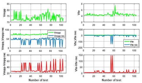
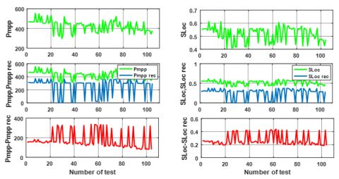
According to Table 4, it is clear that the diagnostic indicators (Vmpp, Vte, Mppf, Rse, FF) have a high sensitivity to the appearance of shading defects, if we take the Vmpp parameter as an example, it has a PRD value of 84.06% and a correlation value Corr= 0.653, these values always belong to the interval PRD=[74, 97.58] and Corr=[0.250, 0.70]. Figures 12, 13 and 14 explain more the high sensitivity of these indicators.
Figure 12 clearly illustrates the high sensitivity of the Vmpp indicator, the plot at the top in green color shows the evolution of the Vmpp(V) parameter in the healthy state in function of number of tests, it is seen that the Vmpp(V) indicator has a value between 70 and 80 volts, the plot at the middle in green illustrates the evolution of Vmpp(V) without fault and the (Vmpprec) in the presence of a shading fault (blue plot), the presence of shading fault from test number 20 to test number 100 has caused a decrease that reaches 0 volts in the voltage value of the three PV panels.
Figure 12. The high sensitivity to the shading fault of the Vmpp and Vte indicators
The plot at the bottom in red color shows the difference between Vmpp(V) in the healthy state and the Vmpprec(V) in the faulty state (Vmpp – Vmpprec), it’s seen that the error is very big from the appearance moment of the fault (test number 20) until test number 100, this large difference (error) is explained by a low correlation of Corr = 0.653 and a big error of PRD = 84.06%.
In the same way as for the Vmpp(V) indicator, the three plots on the right of Figure 12 show the evolution of the Vte indicator in the healthy state (green plot at the top), the evolution of Vte in the healthy state and the failed state (blue plot) and the difference (Vte-Vterec) in red plot, the big difference (error) is explained by a big PRD = 96.92% and a very low correlation corr = 0.397.
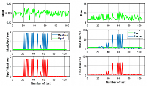
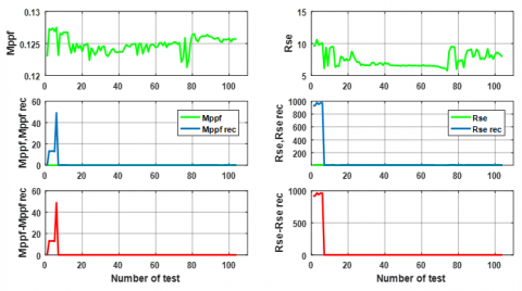
Figure 13. The high sensitivity to the shading fault of the Mppf and Rse indicators
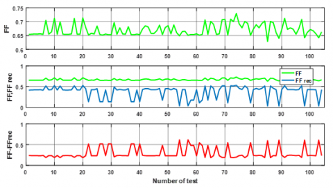
Figure 14. The high sensitivity to the shading fault of the FF indicator
Figures 13 and 14 also illustrate the high sensitivity of the three parameters (Mppf, Rse, FF). The most important is often the difference between each parameter in the healthy state and the same parameter in the presence of a shading fault (red plots). This difference is always explained by a low correlation and a very big PRD (Table 3).
b) Medium sensitivity:
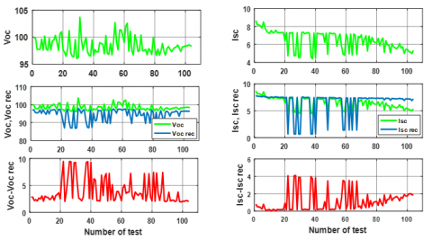
The medium sensitivity to the shading defect of the parameters Voc(V), Isc(I), Impp(I) and SLsc is explained in the same way as the high sensitivity. The most important is often the difference or the error between the indicator without fault and the same indicator in the presence of fault (Voc –Voc rec) and (Isc -Isc rec), the difference is translated by an average correlation Corr=0.766 and PRD=73.51% for Voc(V) and an average correlation Corr=0.703 and PRD=73.56% for Isc(I) (red plots in Figure 15).
Figure 15. The medium sensitivity to shading fault of the Voc and Isc indicators
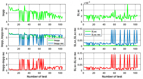
Figure 16. The Medium sensitivity to shading fault of the Impp and SLsc indicator
Figure 16 also illustrates the medium sensitivity to the shading defect of the two parameters (Impp, SLsc) the most important is often the difference between each parameter in the healthy state and the same parameter in the presence of a shading fault (red plots), the difference is always explained by an average correlation and an average PRD error (Table 3).
c) Low sensitivity:
The low sensitivity to the shading defect of the Pmpp and SLoc parameters is explained in the same way as the high sensitivity. The most important is often the difference between the indicator without fault and the same indicator in the presence of shading fault (Pmpp –Pmpp rec) and (SLoc –SLoc rec), this difference is translated by a correlation close to 1 Corr=0.846 and PRD=68.15% for Pmpp indicator and a correlation close to 1 Corr=0.901 and PRD=35.60% for Sloc indicator (red plots in Figure 17).
Figure 17. The low sensitivity to the shading defect of the Pmpp and SLoc indicators
10.2 Connection resistance fault
a) High sensitivity:
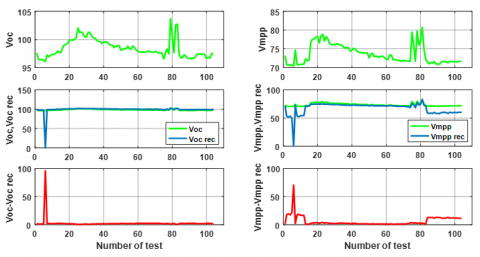
From Table 4 it is clear that the diagnostic indicators (Voc, Vmpp, Mppf, Rse, Isc) have a high sensitivity to the appearance of a resistive fault (connection resistance fault), if we take the Voc parameter as an example, it has a value of PRD = 97.58% and a correlation value Corr = 0.250, these values always belong to the interval PRD= [74, 97.58] and Corr= [0.250, 0.70]. Figures 18, 19 and 20 further explain the high sensitivity of these indicators.
Figure 18. The high sensitivity to the resistive fault of the Voc and Vmpp indicator
Figure 18 clearly illustrates the high sensitivity of the Voc(V) indicator, the plot at the top in green color shows the evolution of the Voc(V) parameter in the healthy state, it’s seen that the Voc indicator has a value between 95 and 105 Volts, the plot at the middle in green color illustrates the evolution of Voc without defect and the Voc rec(V) in the presence of a resistive fault (in blue color), the presence of a resistive fault (blue plot) has caused a decrease which reaches 0 volts in the voltage value of the three PV modules.
The plot at the bottom in red color shows the difference between Voc(V) in the healthy state and Voc rec(V) in the faulty state (Voc - Voc rec), this difference is explained by a low correlation Corr= 0.250 and a very big error of PRD=97.58%
In the same way as for the Voc(V) indicator, the three plots on the right of Figure 18 show the evolution of the Vmpp(V) indicator in the healthy state (at the top in green color), the evolution of Vmpp(V) in the healthy state and the faulty state in blue plot and the difference (Vmpp – Vmpp rec) in red plot. This difference is explained by a very big PRD = 92.17% and a low correlation Corr = 0.644.
Figure 19. The high sensitivity to the resistive fault of the Mppf and the Rse indicators
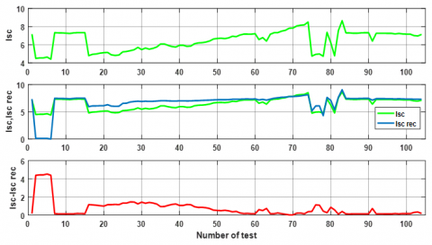
Figure 20. The high sensitivity to the resistive fault of the Isc indicator
Figures 19 and 20 also illustrate the high sensitivity of the three parameters (Mppf, Rse, Isc), the most important is often the difference between each parameter in the healthy state and the same parameter in the faulty state (resistive fault) in red plot, the difference is always explained by a low correlation and a very big PRD (Table 3).
b) Medium sensitivity:
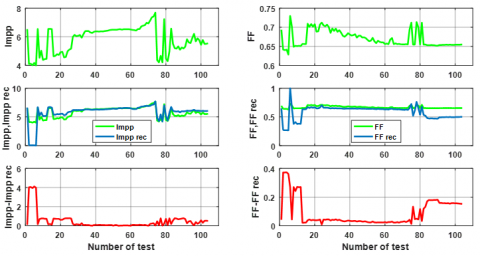
In the same way as for high sensitivity, we explain the medium sensitivity to the resistive fault of Impp and FF parameters, the most important is often the difference between the indicator without fault and the same indicator in the presence of fault (Impp- Impp rec) and (FF-FFrec) presented by (red plots Figure 21), this difference is translated by an average correlation of Corr=0.738, PRD=73.61% for Impp, and Corr=0.742, PRD=70.31% for FF.
Figure 21. The medium sensitivity to the resistive fault of the Impp and FF indicators
c) Low sensitivity:
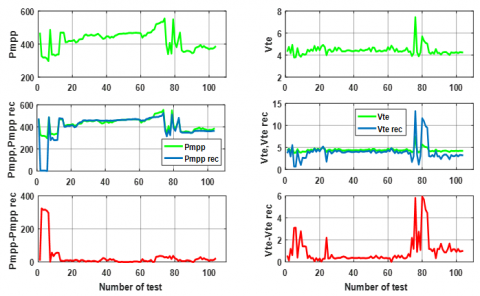
The low sensitivity to the resistive fault of the (Pmpp, Vte, SLsc and SLoc) parameters is presented, the most important is often the difference between the indicator without fault and the same indicator in the presence of fault (Pmpp - Pmpp rec) and (Vte -Vte rec) presented in (red plot Figure 22), this difference is translated by a correlation close to 1 Corr=0.834 and PRD=70.01%for Pmpp and a correlation close to 1 Corr=0.912 and PRD=34.52% for Vte.
Figure 22. The low sensitivity to resistive fault of the Pmpp and Vte indicators
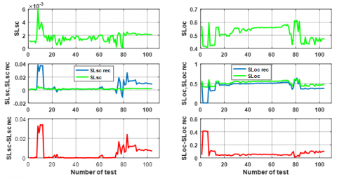
Figure 23. The low sensitivity to the resistive fault of SLsc and Sloc indicators
Figure 23 illustrates the low sensitivity of the two (SLsc, Sloc) parameters, the very important is the difference between each parameter in the healthy state and the same parameter in the presence of a resistive fault (red plots), this difference is explained by a better correlation close to 1 and a low value of the PRD.
The analysis of the obtained results allowed us to conclude that certain diagnostic indicators which belong to the interval of high sensitivity in the case of a shading fault have become belonging to the interval of medium sensitivity or low sensitivity in the case of a resistive fault, taking as an example the Vte and FF parameters, these two parameters have a high sensitivity in the case of a shading fault, however in the case of a resistive fault the Vte parameter has a low sensitivity and the FF has a medium sensitivity, it can also be distinguished that in the case of resistive fault, the Voc and Isc parameters have a high sensitivity, but in the case of shading fault, it has a medium sensitivity, there is also a change in the sensitivity between the SLsc and SLoc parameters.
The proposed residual method in the first part, allowed us to obtain very satisfactory results to the online detection and offline identification faults in the PV generator, the obtained results, also allowed us to determine the intervals confidence and the samples are within or outside these limits. Therefore, the decision of the presence of the defect or not can be made.
The application of SEA method in the second part, allowed us to increase the comparison performance between the diagnostic indicators without faults and the diagnostic indicators in the presence of faults (shading and resistive defects) and it gave us a better sensitivity analysis, in which we classified the diagnostic indicators according to their degree of sensitivity to three main classes high, medium and low sensitivity. The classification is very important, especially to detect and identify the type of defect as quickly as possible, so we can only follow the indicators that have a high sensitivity to be easy and quick to detect and identify the type of fault. The rapid detection and identification of faults in a PV system, gives the possibility to rapid intervention on site to correct the fault and avoid further damage. Therefore reduce the maintenance cost and increase the yield of the PV system.
In perspective we hope to apply the residual and the SEA methods on the rest of defects; by-pass diode faults, connection line faults, short circuited sub- strings, also develop a monitoring and diagnostic system which is able to detecting and identifying as quickly as possible the faults that may occur in the PV system.
[1] Bun, L. (2011). Detection et localisation de défauts pour un système PV, laboratoire G2ELAB dans l’école doctorale EEATS, Université de Grenoble, France. https://www.theses.fr/2011GRENT111.pdf.
[2] Hachana, O., Tina, G.M., Hemsas, K.E. (2016). PV array fault Diagnostic Technique for BIPV systems, Energy and Buildings, 126: 263–274. https://doi.org/10.1016/j.enbuild.2016.05.031
[3] Spataru, S., Sera, D., Kerekes, T., Teodorescu, R. (2015). Diagnostic method for photovoltaic systems based on light I–V measurements. Solar Energy, 119: 29–44. http://dx.doi.org/10.1016/j.solener.2015.06.020
[4] Ali, M.H., Rabhi, A., El Hajjaji, A. (2017). Real time fault detection in photovoltaic systems. Energy Procedia, 111: 914-923. https://doi.org/10.1016/j.egypro.2017.03.25
[5] Belyaev, A., Polupan, O., Dallas, W., Ostapenko, S., Hess, D., Wohlgemuth, J. (2006). Crack detection and analyses using resonance ultrasonic vibrations in full-size crystalline silicon wafers. Applied Physics Letters, 88: 119071-119073. https://doi.org/10.1063/1.2186393
[6] Gokmen, N., Karatepe, E., Celik, B., Silvestre, S. (2012). Simple diagnostic approach for determining of faulted PV modules in string based PV arrays. Solar Energy, 85: 3364-3377. https://doi.org/10.1016/j.solener.2012.09.007
[7] Hu, Y., Gao, B., Song, X., Tian, G.Y., Li, K., He, X. (2013). Photovoltaic fault detection using a parameter based model. Solar Energy, 96: 96-102. https://doi.org/10.1016/j.solener.2013.07.004
[8] Wang, M.H. (2013). A novel extension decision-making method for selecting solar power systems. International Journal of Photoenergy, 108981, 6. https://doi.org/10.1155/2013/108981
[9] Syafaruddin, S., Karatepe, E., Hiyama, T. (2011). Controlling of artificial neural network for fault diagnosis of photovoltaic array. International Conference on Intelligent System Application to Power System, Hersonissos, Greece, 1-6. https://doi.org/10.1109/ISAP.2011.6082219
[10] Zhao, Y., de Palma, J.F., Mosesian, J., Lyons, R., Lehman, B. (2013). Line fault analysis and protection challenges in solar photovoltaic arrays. IEEE Transactions on Industrial Electronics, 60: 3784-3795. https://doi.org/10.1109/TIE.2012.2205355
[11] Drews, A., de Keizer, A.C., Beyer, H.G., Lorenz, E., Van Sark, W.G.J.H.M., Heydenreich, W., Wiemken, E., Toggweiler, P., Bofinger, S., Schneider, M., Heilscher, G., Betcke, J., Stettier, S., Heinemann, D. (2007). Monitoring and remote failure detection of grid-connected PV systems based on satellite observations. Solar Energy, 81: 548-564. https://doi.org/10.1016/j.solener.2006.06.019
[12] Munaz, M.A., Alonso-Garica, M.C., Vela, N., Chenlo, F. (2011). Early degradation of silicon PV modules and guarantly conditions. Solar Energy, 85: 2264-2274. https://doi.org/10.1016/j.solener.2011.06.011
[13] Chouder, A., Silvestre, S. (2010). Automatic supervision and fault detection of PV systemsbased on power losses analysis. Energy Conversion and Management, 51: 1929-1937. https://doi.org/10.1016/j.enconman.2010.02.025
[14] Chine, W., Mellit, A., MassiPavan, A., Kalogirou, S.A. (2014). Fault detection method for grid-connected photovoltaic plants. Renewable Energy, 66: 99-110. https://doi.org/10.1016/j.renene.2013.11.073
[15] Takashima, T., Yamaguchi, J., Otani, K., Ozeki, T., Kato, K., Ishida, M. (2009). Experimental studies for fault location in PV module strings. Solar Energy Materials and Solar Cells, 93: 1079-1082. https://doi.org/10.1016/j.solmat.2008.11.060
[16] Johnson, J., Kuszmaul, S., Bower, W., Schoenwald, D. (2011). Using PV module and line frequency response data to create robust arc fault detectors. In Proceedings of the 26th European Photovoltaic Solar Energy Conference and Exhibition, September 5-9, Hamburg, Germany, pp. 3745-3750. https://doi.org/10.4229/26thEUPVSEC2011-4AV.3.24
[17] Chao, K.H., Ho, S.H., Wang, M.H. (2008). Modeling and fault diagnosis of a photovoltaic system. Electric Power Systems Research, 78: 97-105. https://doi.org/10.1016/j.epsr.2006.12.012
[18] Ducange, P., Fazzolari, M., Lazzerini, B., Marcelloni, F. (2011). An intelligent system for detecting faults in photovoltaic fields. 11th International Conference on Intelligent Systems Design and Application, Cordoba, Spain, 1341-1346. https://doi.org/10.1109/ISDA.2011.6121846
[19] Vergura, S., Aacciani, G., Amoruso, V., Patron, G., Vacca, F. (2009). Descriptive and inferential statistics for supervising and monitoring the operation of PVplants. IEEE Transactions on Industrial Electronics, 56: 4456-4464. https://doi.org/10.1109/TIE.2008.927404
[20] Platon, R., Martel, J., Woodruff, N., Chau, T.Y. (2015). Online fault detection in PV systems. IEEE Transactions on Sustainable Energy, 6: 1200-1207. https://doi.org/10.1109/TSTE.2015.2421447
[21] Xu, P., Hou, J.M., Yuan, D.K. (2013). Fault diagnosis for building grid-connected photovoltaic system based on analysis of energy loss. Advanced Materials Research, 805-806: 93-98. https://doi.org/10.4028/www.scientific.net/AMR.805-806.93
[22] Chao, K-H., Ho, S-H., Wang, M.H. (2008). Modeling and fault diagnosis of a photovoltaic system. Electric Power Systems Research, 78: 97-105. https://doi.org/10.1016/j.epsr.2006.12.012
[23] Spataru, S., Sera, D., Kerekes, T., Teodorescu, R. (2015). Diagnostic method for photovoltaic systems based on light I-V measurements. Solar Energy, 119: 29-44. https://doi.org/10.1016/j.solener.2015.06.020
[24] Swingler, A. (2010). Photovoltaic string inverters and shade-tolerant and maximum power point tracking: Toward optimal harvest efficiency and maximum ROI. Schneider Electric, Burnaby, Canada.
[25] Tina, G.M., Cosentino, F., Ventura, F. (2016). Monitoring and diagnostics of photovoltaic power plants. In Ali Sayigh (Ed.), Renewable Energy in the Service of Mankind (pp. 505-516). Springer International. https://doi.org/10.1007/978-3-319-18215-5_45
[26] Silvestre, S., Kichou, S., Chouder, A., Nofuentes, G., Karatepe, E. (2015). Analysis of current and voltage indicators in grid connected PV systems working in faulty and partial shading conditions. Energy, 86: 42-50. https://doi.org/10.1016/j.energy.2015.03.123
[27] Metatla, A., Benzahioul, S., Bahi, T., Lefebvre, D. (2011). On-line current monitoring and application of a residual method for eccentricity fault detection. Advances in Electrical and Computer Engineering, 11: 85-90. https://doi.org/10.4316/AECE.2011.01011
[28] Boucheham, B. (2008). Matching of quasi-periodic time series patterns by exchange of block-sorting signatures. Pattern Recognition Letters, 29: 501-514. https://doi.org/10.1016/j.patrec.2007.11.004
[29] Hacke, P., Kempe, M., Terwilliger, K., Glick, S., Call, N., Johnston, S., Kurtz, S., Bennett, I., Kloos, M. (2010). Characterization of multicrystalline silicon modules with system bias voltage applied in damp heat. In Proceedings of the 25th European Photovoltaic Solar Energy Conference and Exhibition, September 6-10, Valencia, Spain, pp. 3760-3765. https://doi.org/10.4229/25thEUPVSEC2010-4BO.9.6
[30] Contribution au diagnostic des défauts dans les systèmes photovoltaïques. http://dspace.univ-eloued.dz/handle/123456789/12272