Nitin Kumar Mishra![]() | Ranu*
| Ranu*![]()
© 2023 IIETA. This article is published by IIETA and is licensed under the CC BY 4.0 license (http://creativecommons.org/licenses/by/4.0/).
OPEN ACCESS
We have framed an inventory replenishment model under a finite planning horizon in which replenishment cycle time and replenishment cycle length are different and don’t repeat. The finite planning horizon for different replenishment times and cycle lengths is a real-life scenario. Nowadays, every manufacturing industry wants to achieve maximum profit at a low cost. It is very difficult to maintain the optimal level of inventory, total cost, replenishment time, and replenishment cycle. Along with the health of people, increasing carbon emission also has a dangerous effect on today’s business environment. Therefore, this article analyses an optimal inventory replenishment policy and carbon emission due to deteriorating material and refrigeration while taking into account time, emission-dependent, and inventory-dependent quadratic demand. Materials deterioration affects a large and varied spectrum of business. Therefore, Material that suffers deterioration is considered. Shortage, some lost sales, and partial backlogging are also considered. Backlogging is dependent on the frequency of the waiting period for the next replenishment over a given finite time horizon and fluctuating replenishment cycle. The model has been developed theoretically. Also, a mathematical formulation has been obtained to find the optimal solution to the problem. Following the algorithm, a numerical illustration and a comparative evaluation are explained, along with a sensitivity analysis of each parameter. The tabular and graphical representations of sensitivity analysis were addressed using the Mathematica application version 12.
supply chain management, deterioration, stock-dependent demand, quadratic carbon emission, time demand, a lost sale, shortages, backlog
In recent years, there has been a lot of discussion about inventory systems that emit carbon and degrade the environment. Carbon emissions have been triggering global warming for many years, which has garnered considerable attention. Carbon emission gases, such as carbon dioxide and methane, heat our planet and lead to global warming. To learn more about this, we can visit the page on Climate Change Indicators: Atmospheric Concentrations of Greenhouse Gases. Global warming produces considerable environmental harm because of its destructive, pervasive, and long-term consequences. It is quickly destroying our planet's biodiversity, ultimately causing the extinction of countless plant and animal species. Global warming also causes sea-level rise, ozone layer depletion, rising global temperatures, extreme weather conditions, drought, and flooding. Due to increasingly powerful and frequent severe weather events, global climate change and the greenhouse effect have received a lot of attention. The Paris Protocol, also known as Cap-and-Trade, was created to lessen the greenhouse effect. Under the carbon tax, companies are paid a fixed sum for every tonne of emissions they generate, while the cap-and-trade policy issues a specified number of emissions allowances per year under the cap-trade program [1, 2].
There is growing agreement that Carbon emissions from enterprise economic activities are increasingly being blamed for serious climate change and global warming. Furthermore, reducing a polluted environment is one of the most considerable economic benefits of lowering carbon emissions, and it is becoming a big worry for nations worldwide. Only a few of them consider environmental issues in supply chain management, which include reducing carbon emissions. To reduce carbon emissions, the government of any nation and several regulatory bodies have developed carbon emission programs. The primary regulatory policy is a carbon tax. A carbon tax is charged or imposed by various government agencies on commercial enterprises or businesses that create carbon dioxide throughout their production process and generate environmental destruction [3]. The primary goal of the government entities responsible for taxation is to prevent global warming and safeguard the environment. In other terms, the carbon tax is a cost levied on corporations that use harmful raw materials, such as fossil fuels, in their manufacturing process and transportation, and they are blamed for global warming. Also, a carbon tax can prevent environmental degradation and total cost of Inventory model [4].
Chen et al. investigated an emissions inventory issue using the EOQ model and carbon schemes such as carbon tax, cap, and cap-and-offset [4]. Analyzed the influence of the credit period and environmental policies on inventory management, whenever the credit period has an impact on the demand rate [5]. Determined the optimum lot size and emissions with two of the most commonly used carbon policies to reduce carbon emissions: cap-and-trade and carbon tax [6]. It is investigated that the combined price and production of various commodities in the context of the carbon tax and cap-and-trade legislation. This report considers the joint decisions of retailers concerning inventory supplies and the reducing carbon emission investments model, taking into consideration the three carbon regulatory policies. In particular, it expands the economic quantitative order model to take into account the supply of carbon decreasing expenditure, in addition to complying with the carbon cap, price, and trade policies [7]. Based entirely on the EOQ model, the researcher discusses production lot-sizing problems under the carbon tax, cap, and carbon trade norms. From the previous research study, it is known that there is very little study on carbon emission in finite planning. Therefore, I have decided to focus on it in my work.
Obsolescence, damage, and depreciation can all cause on-hand inventory to deteriorate over time, resulting in lost sales, decreased earnings, and poorer customer satisfaction. The variable fraction value of on-hand inventory represents the proportion of total inventory that is prone to deterioration over time. Managing the supply chain for goods that deteriorate and emit carbon is difficult and risky because the utility of such products can decline due to spoilage, damage, or degradation during storage or transport. Carbon emissions and deterioration mostly occur due to global warming. Many countries are increasingly focusing on reducing greenhouse gas emissions and environmental devastation, employing pivotal methods such as carbon caps and taxes to accomplish this task. Researchers examined an integrated supply chain model for a single supplier and a single buyer manufacturing stock, taking into consideration imperfect output, including reworked products, and various governmental mechanisms for decarbonization, such as a carbon tax, carbon cap-and-trade, and item deterioration, all at the same time. They developed a multi-objective framework to minimize the overall cost and emissions simultaneously. The demand for a product is generally influenced by several uncontrollable factors such as pricing, season, time, accessibility, and so on. However, addressing a fuzzy demand rather than static demand is considered [8]. Through an EOQ model, we know that retailers or buyers pay a constant carbon tax, and buyers can use one of three forms of payment to pay: cash payment, advance payment, or credit payment [9]. Credit transactions seem to be the most economical and effective of the multiple payment alternatives for lowering carbon emissions and maintaining the environment. They also state that items deteriorate over time and thus can't be sold after their expiry. Researchers addressed a production planning problem for deteriorating items, considering a carbon taxation policy with preservation technology investment [10]. This study also focuses on two carbon pollution schemes: carbon cap policies and the cap-and-trade system. It provides a single-vendor and single-buyer integrated supply chain stock model with decaying goods of inferior quality, considering carbon emissions [11]. Researchers introduced microbes initially forming a film on materials such as metals, and organic biomaterials which leads to the final degradation of the compound. A hot and humid climate catalyzes the process [12]. Due to carbon emissions, the deterioration of anything is more obvious that can’t be ignored. This paper mainly focuses on materials getting deteriorated because of corrosion, rust, rotting along with carbon emission. corrosion or rust are directly related to deterioration but indirectly related to emission. When metal products are manufactured or transported, they often require energy to be produced or moved. Additionally, there is a limited amount of research that specifically examines the relationship between carbon emission policies and asset deterioration over time in inventory control and management, and nobody has considered carbon emission policies with deterioration in a finite planning horizon for unequal cycle length with carbon emission policies.
The main objective is to control carbon emissions and find the optimal solution by considering three models: the carbon cap and tax model, excluding shortage, with partial backlogging, and full backlogging. Carbon emissions and carbon cap and taxes are the fundamental points of this article [3]. Shortages or stock-out scenarios arise in any business or industrial company due to many factors, such as pricing and a high rate of deterioration [13]. In today's scenario, taking stock-out into account in any inventory model is necessary. It is anticipated that when one merchant receives the requested amount from the other merchant, they would satisfy the customers who have been waiting and then stock the remaining items for their regular demand. However, due to their impatience or other sources accessible in the region, not all buyers waiting in line can wait for the supply to arrive, resulting in a proportion of consumers waiting to lead to lost sales. Shortages are therefore defined as partially backlogged. A model permit shortage in all iterations of replenishment except for the final cycle. Each cycle during which shortages are created begins with replenishment and finishes with a backlogged shortage in the final cycle [14]. Furthermore, presented a novel restocking approach where each cycle starts with shortfalls and ends with a positive inventory. Most researchers have considered shortage for a single cycle [15-17] and there was no literature on a shortage of carbon emission and deterioration under finite planning horizons for unequal cycle length.
The significant result of using a time-dependent quadratic demand mechanism is that it accommodates all three forms of demand functions: increasing, falling, or constant, according to demand constants [18]. Researchers introduced a supplier-retailer EOQ stock supply model with quadratic demand dependent on time and stock, as well as partial backlog throughout all cycles during a finite planned period [19]. Some researchers included a quadratic time-dependent demand function for both finite and infinite horizons in their inventory management system [20]. Furthermore, employed the quadratic time demand function in their research study under finite planning of equal replenishment cycles [21]. It is noticeable from the previous analysis that the discussion on deteriorating goods in nature has not been addressed for carbon tax cost and shortage along with carbon-dependent, time-dependent quadratic, and inventory-dependent demand under finite planning horizons for unequal cycle lengths (Table 1).
Table 1. For a review of the above literature
|
Article |
Carbon dependent Demand |
Deterioration |
Inventory dependent |
Time-dependent Quadratic demand |
Carbon Emissions cost |
Shortages |
Finite Planning horizon |
|
Toptal et al. [2] |
× |
× |
× |
× |
✓ |
× |
× |
|
Mishra et al.[3] |
× |
✓ |
× |
× |
✓ |
✓ |
× |
|
Chen et al. [4] |
× |
× |
× |
× |
✓ |
× |
× |
|
Xu et al. [7] |
× |
✓ |
× |
× |
✓ |
× |
× |
|
Sarkar [18] |
× |
✓ |
× |
✓ |
× |
✓ |
✓ |
|
Pushpinder Singh et al. [19] |
× |
✓ |
✓ |
✓ |
× |
✓ |
✓ |
|
Ghosh and Chaudhuri [21] |
× |
✓ |
× |
✓ |
× |
✓ |
✓ |
|
This Paper |
✓ |
✓ |
✓ |
✓ |
✓ |
✓ |
✓ |
1.1 Research gap
So far, multiple researches on material deterioration and emission have already been conducted. Furthermore, neither of the research has considered an inventory management model that incorporates carbon emission measures including a carbon tax, covering degrading materials with emission-dependent, nonlinear time-dependent, and inventory-dependent demand, along with shortage. This is a significant and strong research gap, and the study is especially unique in that the issues highlighted are entirely economic and environmental in scope. Based on the aforementioned research, the authors claim that none of the other researchers has developed a model for managing deteriorating products, incorporating emission-dependent, time-dependent quadratic, and inventory-dependent demand over a finite horizon. Finite planning horizons refer to the period in which decisions about inventory replenishment are made. Longer planning horizons allow for more time to make decisions, potentially leading to longer replenishment cycles, while shorter planning horizons can result in shorter replenishment cycles.
The remaining sections of this article are organized as follows: Section 2 presents a list of all the assumptions and notations used in the study. In Section 3, a mathematical model is presented, and a solution to it is provided. The optimality requirements for cost equations are discussed in section 4, with the help of a theorem and the Mathematica software. Section 5 includes a numerical example, an algorithm for finding ti, si, and total cost in the Mathematica tool, as well as sensitivity analysis, and a comparison discussion with graphs and tables. In Section 6, managerial suggestions are provided. Finally, the conclusions of the proposed model are discussed.
Figure 1. Inventory level with shortage and lost sale
As seen in the inventory Figure 1 for finite planning along with shortages. Differential equation of inventory level besides shortages given by Eq. (1) and Eq. (5) Boundary condition ILi+1 (si+1)=0.
$\begin{aligned} \frac{d I L_{i+1}(t)}{d t}+ & \left(\theta_1+\theta_2\right) I L_{i+1}(t)=-\mathrm{D}(\mathrm{t}) \\ & t_i<\mathrm{t}<s_{i+1}\end{aligned}$ (1)
where, {i=1,2,3…………………. n1}.
Taking θ2=αt and the differential equation's solution is given by:
$\begin{aligned} \frac{d I L_{i+1}(t)}{d t} & =-\mathrm{D}(\mathrm{t})-\alpha t I L_{i+1}(t) \\ t_i & <\mathrm{t}<s_{i+1}\end{aligned}$ (2)
$I L_{i+1}(t)=e^{-\frac{\alpha t^2}{2}-t \theta_1} \int_t^{s_{i+1}} \mathrm{D}(\mathrm{u}) e^{\frac{\alpha u^2}{2}+t} \mathrm{du}$ (3)
$I L_{i+1}(t)=\int_t^{s_{i+1}} \mathrm{D}(\mathrm{u}) e^{\theta_1(u-t)+\frac{\alpha\left(u^2-t^2\right)}{2}} \mathrm{du}$ (4)
$\begin{gathered}I L_{i+1}(t)=\left[\left(1+t \theta_1+\frac{\alpha}{2} t^2\right)\left(t-t_i\right)-\frac{\theta_1}{2}\left(t^2-t_i^2\right)\right. \left.-\frac{\alpha}{6}\left(t^3-t_i^3\right)\right] D(t)\end{gathered}$
The instantaneous level of shortage ILSi+1(t) with the boundary condition ILSi+1(si)=0, is given by the following differential equation:
$\frac{d I L S_{i+1}(t)}{d t}=D(t) \beta(t) \quad$ where $s_i<\mathrm{t}<t_i$ (5)
$\begin{gathered}\frac{d I L S_{i+1}(t)}{d t}=\frac{D(t)}{\delta\left(t_i-t\right)+1} \\ I L S_{i+1}(t)=\int_{s_i}^{t_i} \frac{D(t)}{\delta\left(t_i-t\right)+1} d t=\frac{D(t)\left(t_i-t\right)}{\delta\left(t_i-t\right)+1}\end{gathered}$ (6)
So total amount of inventory held during the interval held during the $\left[t_i, s_{i+1}\right]$
$R_{i+1}=\int_{t_i}^{s_{i+1}}\left\{\int_t^{s_{i+1}} \mathrm{D}(\mathrm{u}) e^{\theta_1(u-t)+\frac{\alpha\left(u^2-t^2\right)}{2}} \mathrm{du}\right\} \mathrm{dt}$ (7)
We may express Eq. (7) as below by changing the position of integration and skipping the higher powers of α2.
$\begin{aligned} R_{i+1}=\int_{t_i}^{s_{i+1}}\{(1+ & \left.\theta_1 t+\frac{\alpha}{2} t^2\right)\left(t-t_i\right) \\ & -\frac{\theta_1}{2}\left(t^2-t_i{ }^2\right) \\ & \left.-\frac{\alpha}{6}\left(t^3-t_i{ }^3\right)\right\} D(t) d t\end{aligned}$ (8)
The total amount of that quantity for which customers are waiting i.e., the amount of shortage during the interval $\left[s_i, t_i\right]$. After rearranging the ordering, $S_{i+1}$ can be given as:
$S_{i+1}=\int_{s_i}^{t_i} I L S_{i+1}(t) d t$$=\int_{s_i}^{t_i}\left\{\int_{s_i}^{t_i} \frac{D(u)}{\delta\left(t_i-u\right)+1} d u\right\} d t$$=\int_{s_i}^{t_i} \frac{\left(t_i-t\right) D(t)}{\delta\left(t_i-t\right)+1} d t$ (9)
The total order quantity for a finite planning horizon.
$\mathrm{Q}=\sum_{i=1}^n Q_{i+1}=\sum_{i=1}^n\left\{R_{i+1}+S_{i+1}\right\}$
$Q_{i+1}=\int_{t_i}^{s_{i+1}}\left\{\left(1+\theta_1 t+\frac{\alpha}{2} t^2\right)\left(t-t_i\right)-\frac{\theta_1}{2}\left(t^2-t_i^2\right)\right.$$\left.-\frac{\alpha}{6}\left(t^3-t_i^3\right)\right\} D(t) d t$$+\int_{s_i}^{t_i} \frac{\left(t_i-t\right) D(t)}{\delta\left(t_i-t\right)+1} d t$
The total number of deteriorated components throughout each replenishment is as follows:
$D_{i+1}=\int_{s_i}^{t_i} \theta_2 I L_{i+1}(t) d t$
$\begin{gathered}=\alpha t\left\{\int_{t_i}^{s_i}\left(1+\theta_1 t+\frac{\alpha}{2} t^2\right)\left(t-t_i\right)-\frac{\theta_1}{2}\left(t^2-t_i^2\right)\right. \left.-\frac{\alpha}{6}\left(t^3-t_i^3\right) D(t) d t\right\}\end{gathered}$ (10)
In the cases of some materials, the Buyer can generally not wait for some product, so only a proportion β(φ) of the demand during the stock-out duration is backlogged, where φ is the amount of time the buyer waits for the quantity of negative inventory. Therefore, the leftover proportion (1-β(φ)) is lost. Sarkar et al. [18], the amount has become lost during the interval $\left[s_i, t_i\right]$ is given as:
$L_{i+1}=\int_{s_i}^{t_i}\{D(t)-D(t) \beta(\varphi)\} d t$
$\begin{aligned} & =\int_{s_i}^{t_i}\{(1-\beta(\varphi)) D(t)\} d t \\ & =\int_{s_i}^{t_i}\left\{\delta \frac{\left(t_i-t\right) D(t)}{\delta\left(t_i-t\right)+1}\right\} d t\end{aligned}$ (11)
Amount of Carbon emission cost during the interval [ti, si+1] can be expressed as:
$C e=\sum_{i=0}^{n_1-1} \mathrm{c}^{\hat{}}+\hat{P}_r * R_{i+1}+\widehat{h_c} \int_{t_i}^{s_{i+1}} I L_{i+1}(t) d t$
$\begin{aligned} & C e=\sum_{i=0}^{n_1-1} \mathrm{c}^{\hat{}}+\hat{P}_r * Q_{i+1} \\ &+\widehat{h_c} \int_{t_i}^{s_{i+1}}\left\{\int_t^{s_{i+1}} \mathrm{D}(\mathrm{u}) e^{\theta_1(u-t)+\frac{\alpha\left(u^2-t^2\right)}{2}} \mathrm{du}\right\} d t\end{aligned}$
The amount of CO2 emissions from refrigeration systems is influenced by factors like refrigerant type, energy efficiency, usage frequency, system size, and power source. Usage of fossil fuels leads to higher emissions while energy-efficient technologies and smaller systems result in lower CO2 emissions. According to researchers, the total cost of Carbon emission cost/carbon tax during the interval $\left[t_i, s_{i+1}\right]$ can be expressed as [22]:
$\begin{aligned} & C e=\tau\left\{\sum_{i=0}^{n_1-1}{c}^{\hat{}}+\hat{P}_r \int_{t_i}^{s_{i+1}}\left\{\left(1+\theta_1 t+\frac{\alpha}{2} t^2\right)\left(t-t_i\right)-\frac{\theta_1}{2}\left(t^2-t_i^2\right)\right.\right. \\ & \left.-\frac{\alpha}{6}\left(t^3-t_i{ }^3\right)\right\} D(t) d t \\ & +\int_{s_i}^{t_i} \frac{\left(t_i-t\right) D(t)}{\delta\left(t_i-t\right)+1} d t \\ & \left.+\widehat{h_c} \int_{t_i}^{s_{i+1}}\left\{\int_t^{s_{i+1}} \mathrm{D}(\mathrm{u}) e^{\theta_1(u-t)+\frac{\alpha\left(u^2-t^2\right)}{2}} \mathrm{du}\right\} d t\right\} \\ & \end{aligned}$ (12)
Total cost = Replenishment cost + Stock holding cost + purchasing cost + Deteriorating cost + Storage cost + Lost sale cost + Carbon emission cost+ Transportation cost.
$\operatorname{TCR}\left(t_i, s_i, n_1\right)=n_1 * O_r \mathrm{z}+\sum_{i=0}^{n_1-1} H \int_{t_i}^{s_{i+1}} I L_{i+1}(t) d t+\sum_{i=0}^{n_1-1} W_h * Q_{i+1}$
$+\sum_{i=0}^{n_1-1} D_t * \theta_2 \int_{t_i}^{s_{i+1}} I L_{i+1}(t) d t+\sum_{i=0}^{n_1-1} s \int_{s_i}^{t_i} I L S_{i+1}(t) d t$
$+\sum_{i=0}^{n_1-1} l \int_{s_i}^{t_i}\left\{\delta \frac{\left(t_i-t\right) D(t)}{\delta\left(t_i-t\right)+1}\right\} d t+\sum_{i=0}^{n_1-1} \mathrm{c}^{\wedge}+\hat{P}_r Q_{i+1}$
$+\widehat{h_c} \int_{t_i}^{s_{i+1}} I L_{i+1}(t) d t$
$\operatorname{TCR}\left(t_i, s_i, n_1\right)=n_1 * O_r$$+\sum_{i=0}^{n_1-1} H \int_{t_i}^{s_{i+1}} I L_{i+1}(t) d t+\sum_{i=0}^{n_1-1} W_h * Q_{i+1}$
$+\sum_{i=0}^{n_1-1} D_t * \alpha t \int_{t_i}^{s_{i+1}} I L_{i+1}(t) d t$$+\sum_{i=0}^{n_1-1} s \int_{s_i}^{t_i} I L S_{i+1}(t) d t$
$+\sum_{i=0}^{n_1-1} l \int_{s_i}^{t_i}\left\{\delta \frac{\left(t_i-t\right) D(t)}{\delta\left(t_i-t\right)+1}\right\} d t$
$+\sum_{i=0}^{n_1-1}\mathrm{c}^{\hat{}}+\hat{P}_r\left\{R_{i+1}+\int_{s_i}^{t_i} I L S_{i+1}(t) d t\right\}$$+\widehat{h_c} \int_{t_i}^{s_{i+1}} I L_{i+1}(t) d t$
$\operatorname{TCR}\left(t_i, s_i, n_1\right)=n_1 * O_r+\sum_{i=0}^{n_1-1}\left\{H+\tau \widehat{h_c}\right\} \int_{t_i}^{s_{i+1}} I L_{i+1}(t) d t$
$+\sum_{i=0}^{n_1-1} D_t * \alpha t \int_{t_i}^{s_{i+1}} I L_{i+1}(t) d t$$+\left\{W_h+\tau \hat{P}_r\right\} \sum_{i=0}^{n_1-1} Q_{i+1}$
$+\{s+l \delta\} \sum_{i=0}^{n_1-1} \int_{s_i}^{t_i} I L S_{i+1}(t) d t+{c}^{\hat{}}$
$\operatorname{TCR}\left(t_i, s_i, n_1\right)=n_1 * O_r+\sum_{i=0}^{n_1-1}\left(H+\tau \widehat{h_c}\right) \int_{t_i}^{s_{i+1}} I L_{i+1}(t) d t$
$+\sum_{i=0}^{n_1-1} D_t * \alpha t \int_{t_i}^{s_{i+1}} I L_{i+1}(t) d t$
$+\left\{W_h+\tau \hat{P}_r\right\} \sum_{i=0}^{n_1-1}\left(R_{i+1}+S_{i+1}\right)$
$+\left(s+\tau \hat{P}_r+l \delta\right) \sum_{i=0}^{n_1-1} \int_{s_i}^{t_i} I L S_{i+1}(t) d t+\tau \mathrm{c}^{\hat{}}$
$\operatorname{TC}\left(t_i, s_i, n_1\right)=n_1 * O_r$$+\sum_{i=0}^{n_1-1}\left(H+\tau \widehat{h_c}\right) \int_{t_i}^{s_{i+1}} I L_{i+1}(t) d t$
$+\sum_{i=0}^{n_1-1} D_t * \alpha t \int_{t_i}^{s_{i+1}} I L_{i+1}(t) d t$$+\left\{W_h+\tau \hat{P}_r\right\} \sum_{i=0}^{n_1-1} R_{i+1}$
$+\left(s+W_h+\tau \hat{P}_r+l \delta\right) \sum_{i=0}^{n_1-1} \int_{s_i}^{t_i} I L S_{i+1}(t) d t+\tau {c}^{\hat{}}$
$\mathrm{TC}\left(t_i, s_i, n_1\right)=n_1 * O_r+\sum_{i=0}^{n_1-1}\left(H+\tau \widehat{h_c}\right) \int_{t_i}^{s_{i+1}} \int_t^{s_{i+1}} \mathrm{D}(\mathrm{u}) e^{\theta_1(u-t)+\frac{\alpha\left(u^2-t^2\right)}{2}} \mathrm{du} d t$
$+\sum_{i=0}^{n_1-1} D_t * \alpha t \int_{t_i}^{s_{i+1}} \int_t^{s_{i+1}} \mathrm{D}(\mathrm{u}) e^{\theta_1(u-t)+\frac{\alpha\left(u^2-t^2\right)}{2}} \mathrm{du} d t$
$+\left\{W_h+\tau \hat{P}_r\right\} \sum_{i=0}^{n_1-1} R_{i+1}$
$+\left(s+W_h+\tau \hat{P}_r+l \delta\right) \sum_{i=0}^{n_1-1} \int_{s_i}^{t_i} I L S_{i+1}(t) d t+{c}^{\hat{}}$
$\operatorname{TC}\left(t_i, s_i, n_1\right)=n_1 * O_r+\sum_{i=0}^{n_1-1}\left(H+\tau \widehat{h}_c+W_h+\tau \hat{P}_r\right) \int_{t_i}^{s_{i+1}}\left[\left(1+t \theta_1+\frac{\alpha}{2} t^2\right)\left(t-t_i\right)-\frac{\theta_1}{2}\left(t^2-t_i^2\right)-\frac{\alpha}{6}\left(t^3-t_i^3\right)\right] D(t) d t$
$+\sum_{i=0}^{n_1-1} D_t \int_{t_i}^{s_{i+1}} \alpha t\left\{\left(1+\theta_1 t+\frac{\alpha}{2} t^2\right)\left(t-t_i\right)-\frac{\theta_1}{2}\left(t^2-t_i^2\right)-\frac{\alpha}{6}\left(t^3-t_i^3\right)\right\} D(t) d t$
$+\left(s+W_h+\tau \hat{P}_r+l \delta\right) \sum_{i=0}^{n_1-1} \int_{s_i}^{t_i} \frac{\left(t_i-t\right) D(t)}{\delta\left(t_i-t\right)+1} d t+\tau {c}^{\hat{}}$
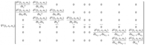
The objective is that the fundamental values of ti and si must be determined to reduce the total variable cost TC of the stock control and management. The requirements to find the values of to ti and si are given below:
$\begin{aligned} & \frac{\partial T C\left(t_i, s_i, n_1\right)}{\partial t_i}=0 \\ & \frac{\partial T C\left(t_i, s_i, n_1\right)}{\partial s_i}=0\end{aligned}$
By neglecting $\alpha^2$ and the higher terms of $\alpha$, because $\alpha$ have a negligible value then we get:
$\begin{aligned} \frac{\partial T C\left(t_i, s_i, n_1\right)}{\partial s_i}=\left(H+\tau \widehat{h_c}\right. & \left.+W_h+\tau \hat{P}_r\right)\left[\left(s_i \theta_1+\frac{\alpha}{2} s_i{ }^2+1\right)\left(s_i-t_{i-1}\right)\right. \\ & \left.-\frac{\theta_1}{2}\left(s_i{ }^2-t_{i-1}^2\right)-\frac{\alpha}{6}\left(s_i{ }^3-t_{i-1}^3\right)\right] D\left(s_i\right) \\ & +D_t \alpha s_i\left[\left(s_i \theta_1+1\right)\left(s_i-t_{i-1}\right)\right. \\ & \left.-\frac{\theta_1}{2}\left(s_i{ }^2-t_{i-1}^2\right)\right] D\left(s_i\right) \\ & +\left(s+W_h+\tau \hat{P}_r+l \delta\right)\left[\frac{\left(t_i-s_i\right)}{\delta\left(t_i-s_i\right)+1}\right] D\left(s_i\right)\end{aligned}$ (15)
$\begin{aligned} \frac{\partial T C\left(t_i, s_i, n_1\right)}{\partial t_i}=\left(H+\tau \widehat{h_c}+W_h\right. & \left.+\tau \widehat{P}_r\right) \int_{t_i}^{s_{i+1}}\left[\theta_1\left(t_i-t\right)+\frac{\alpha}{2}\left(t_i^2-t^2\right)-1\right] D(t) d t \\ & +D_t \int_{t_i}^{s_{i+1}} \alpha t\left[\theta_1\left(t_i-t\right)-1\right] D(t) d t \\ & +\left(s+W_h+\tau \widehat{P}_r+l \delta\right)\left[\int_{s_i}^{t_i} \frac{D(t)}{\delta\left(t_i-t\right)^2+1} d t\right]\end{aligned}$ (16)
$\begin{aligned} \frac{\partial^2 T C\left(t_i, s_i, n_1\right)}{\partial s_i^2}=\frac{1}{6}\left\{\left(H+\tau \widehat{h}_c\right.\right. & \left.+W_h+\tau \widehat{P}_r\right)\left(s_i-t_{i-1}\right)\left[6\left(\theta_1+\alpha s_i\right)\left(a+b s_i+c s_i^2\right)\right. \\ & +\left(3\left(2 s_i \theta_1+\alpha s_i^2+2\right)-3 \theta_1\left(s_i+t_i-1\right)-\alpha\left(s_i^2+t_{i-1}^2\right.\right. \\ & \left.\left.\left.+s_i t_{i-1}\right)\right)\left(a+b s_i+c s_i^2\right)\right] \\ & +3 D_t \alpha\left(s_i-t_{i-1}\right)\left[\left(2-\theta_1 t_{i-1}+\theta_1 s_i\right)\left(b+2 c s_i\right)\right. \\ & \left.+\left(2-\theta_1 t_{i-1}+\theta_1 s_i\right)\left(a+b s_i+c s_i^2\right)\right] \\ & +6\left(s_h+W_h+\tau P_r^{\wedge}+I \delta\right)\left[\frac{\left(t_i-s_i\right)}{1+\delta\left(t_i-s_i\right)}\left(b+2 c s_i\right)\right. \\ & \left.\left.-\frac{1}{1+\delta\left(t_i-s_i\right)^2}\left(a+b s_i+c s_i^2\right)\right]\right\}\end{aligned}$ (17)
$\begin{aligned} \frac{\partial^2 T C\left(t_i, s_i, n_1\right)}{\partial t_i^2}=\left(H+\tau \widehat{h_c}\right. & \left.+W_h+\tau \widehat{P}_r\right) \int_{t_i}^{s_{i+1}}\left(\theta_1+\alpha t_i\right)\left(a+b t+c t^2\right) d t \\ & +\left(H+\tau \widehat{h}_c+W_h+\tau \widehat{P}_r\right)\left(a+b t_i+c t_i^2\right) \\ & +D_t \int_{t_i}^{s_{i+1}} \alpha t \theta_1\left(a+b t+c t^2\right) d t \\ & +D_t \alpha t_i\left(a+b t_i+c t_i^2\right) \\ & -2\left(s+W_h+\tau \hat{P}_r+l \delta\right)\left[\int_{s_i}^{t_i} \frac{\left(a+b t+c t^2\right)}{\left(\delta\left(t_i-t\right)^2+1\right)^2} d t\right]\end{aligned}$ (18)
The sufficient requirement, the Hessian matrix with TC has to be positive definite for TC to be minimum for a fixed n1. Moreover, Theorem proves that TC is positive. Therefore, By the iterative method and using Mathematica software the optimal value of ti and si for a given positive integer n1 may be calculated from the above Eqns. (16) and (17).
Theorem: -
If ti and si satisfy the inequality, (i) $\frac{\partial^2 T C\left(t_i, s_i, n_1\right)}{\partial t_i^2} \geq 0$, (ii) $\frac{\partial^2 T C\left(t_i, s_i, n_1\right)}{\partial s_i^2} \geq 0,(i i i) \frac{\partial^2 T C\left(t_i, s_i, n_1\right)}{\partial t_i^2}-\left|\frac{\partial T c\left(t_i, s_i, n_1\right)}{\partial t_i \partial s_i}\right| \geq 0$ and (iv)$\frac{\partial^2 T C\left(t_i, s_i, n_1\right)}{\partial s_i{ }^2}-\left|\frac{\partial T C\left(t_i, s_i, n_1\right)}{\partial s_i \partial t_i}\right| \geq 0$ for all i = 1, 2,..., n then TC will be positive definite.
The sufficient condition for TC to be minimum for a fixed n1 is that the Hessian matrix with TC has to be positive definite.
Theorem proves that TC is positive. Hence, by utilizing the iterative method and Mathematica software, the optimal values of ti and si for a given positive integer n1 may be calculated from the above Eqns. (16) and (17).
1. The initial step involves assigning constant values to all the given parameters, namely $W_h ; \mathrm{P} ; \mathrm{a} ; \mathrm{b} ; \mathrm{c} ; \theta$, G.
2. The proposed model aims to identify the optimal cost and ordering replenishment strategy, which can be achieved through the following steps:
i. If we will set, $n_1=1$ then $s_1=0, s_2=\mathrm{T}$. Initializing with the parameter's value t1, determine t1 with the help of Eq. (17).
ii. If we take $n_1=2$, then by initializing the value of the $t_{\mathrm{i}}$ taking $\mathrm{s}_0=0$ and $\mathrm{s}_2=\mathrm{T}$. After that, we can calculate $s_2$ by using Eq. (1).
iii. From Eq. (17), find $t_2$ using the calculated values of $\mathrm{t}_1$ and $\mathrm{s}_2$ in the previous step.
iv. By using Eq. (16), Again, taking the values of $\mathrm{t}_2$ and $\mathrm{s}_2$, calculate $s_3$. Trying to continue in this manner until all unique and optimal values of ti and si are obtained for all n1.
v. Having the values of $s_{n_1-1}$ and $t_{n_1-1}$ nearly equal to $\mathrm{T}$ (horizon planning), and the values of $\mathrm{s}_{\mathrm{i}}$ and $\mathrm{t}_{\mathrm{i}}$ are satisfying the theorem of the Hessian matrix.
vi. For each $n_1=1 ; 2 ; 3 ;:::$ we will calculate the unique and optimal values of $\mathrm{t}_{\mathrm{i}}$ and $\mathrm{s}_{\mathrm{i}}$.
3. By using Eq. (10), TC $\left(n_1\right)$ is collected to calculate the optimum total cost value of the system (TC) $\left(n_1\right)$ by using the following condition:
i. For $\mathrm{n} 1=1$ then $\mathrm{TC}=\mathrm{TC}(\mathrm{n} 1)$ and stop. For $\mathrm{n} 1>1$, and if $\mathrm{TC}(\mathrm{n} 1) \leq \mathrm{TC}(\mathrm{n} 1-1)$ and $\mathrm{TC}(\mathrm{n} 1) \leq \mathrm{TC}(\mathrm{n} 1+1)$ then $\mathrm{TC}(\mathrm{n} 1)=$ Optimal (TC) And stop otherwise go to the previous step. Similarly, we can calculate carbon emissions cost and the total quantity.
4.1 Numerical illustration for the proposed model
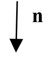
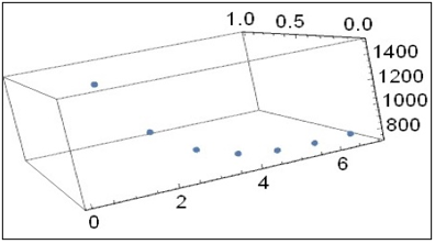
Example 1. $\mathrm{b}=1$ unnit $/ \mathrm{yr}, \mathrm{c}=5$ unit $/ \mathrm{yr}, \mathrm{a}=25$ unit $/ \mathrm{yr}, \alpha=0.001$, $\mathrm{S}=2 \$ /$ unit, $\quad \tau=0.003 \$ /$ ton emission, $\mathrm{h}_{\mathrm{c}}^{\wedge}=0.1$ ton CO2/ unit, $\mathrm{P}_{\mathrm{r}}^{\wedge}=0.030 .1$ ton C02/unit, $\mathrm{D}_{\mathrm{t}}=0.01, \mathrm{~W}_{\mathrm{h}}=0.3 \$ /$ unit, $\mathrm{S}=2 \$$ /unit, $\mathrm{l}=10 \$$ /unit, $\mathrm{H}=4 \$$ /unit/yr, $\alpha=$ $0.001, \delta=4, \theta_1=0.002, \mathrm{~A}=60 \$ /$ order, $\mathrm{T}=4 \quad$. The mathematical calculation tool Mathematica version-12 is used to solve the nonlinear equation systems Eq. (16) and Eq. (17). The optimality of the total system cost and replenishment cycles time can be observed in Table 2, Table 3, Figure 2, and Figure 3 for all values mentioned in the example1, respectively, for all the values mentioned in Example 1. In a finite planning horizon with unequal cycles length that is a real time scenario. Finite planning horizon for unequal cycles length can be observed in Table 3.
4.2 Tables and figures
Table 2. Table for TC for Example 1
|
Qi+1 |
CE |
TC |
|
|
1 |
145.964 |
0.0504865 |
1525.31 |
|
2 |
140.436 |
0.0521384 |
1079.27 |
|
3 |
121.986 |
0.0465045 |
862.14 |
|
4 |
101.422 |
0.0390947 |
756.45 |
|
5 |
41.5876 |
0.0056345 |
711.40 |
|
6* |
71.8061 |
0.0279307 |
700.19 |
|
7 |
62.2117 |
0.0242669 |
709.07 |
Table 3. Optimal strategy for Example 1
|
|
ti |
si |
|
1 |
0.174496 |
0.979947 |
|
2 |
1.10192 |
1.76505 |
|
3 |
1.85751 |
2.4267 |
|
4 |
2.50212 |
3.00571 |
|
5 |
3.07019 |
3.52535 |
|
6* |
3.58222 |
4.000000 |
Figure 2. Proposed 3-D graphic representation
Figure 3. Proposed graphic representation
Replenishment cycles can be observed in Tables 2 and 3, respectively, for all the values mentioned in Example 1.
4.3 Sensitivity analysis and observations
As we are aware, uncertainties and unpredictable market conditions can lead to variations in some parameters' values in decision-making scenarios. Therefore, it is essential to examine the resulting changes in the total cost, emission values, and optimal replenishment cycle. Table 5 presents a comprehensive sensitivity analysis that illustrates how alterations in parameter values can impact the results or outcomes. Hence, in this section, we will analyze the sensitivity level of the total cost and carbon emission cost-optimal solution of the previous Example 1 by changing various system component values. This analysis is carried out using graphical illustrations. Each parameter's value is modified by varying a, b, c, τ, δ, α and θ1 in -50%, -25%, +25%, and +50%, focusing on one parameter at a particular time and keeping the remaining values constant. The optimal solutions for n, TC, and CE are determined in each scenario with the aid of Mathematica software version-12.
4.4 Some exceptional cases
The following are the important exceptional circumstances that impact the optimum current value of total cost. See Table 4 for couplet analysis.
Table 4. Comparison chart for some expectational
|
Some expectational condition |
Replenishment cycle(n*} |
Carbon emission cost |
Time intervals (years) |
Q* Order Quantity |
Total Cost of the system (TC*) |
|
|
ti si |
||||||
|
θ1=0 |
6 |
0.0279 |
0.174335 |
0.980015, |
71.7926 |
716.013 |
|
1.10189 |
1.76513 |
|||||
|
1.85753 |
2.42678 |
|||||
|
2.50215 |
3.00577 |
|||||
|
3.07021 |
3.52538 |
|||||
|
3.58222 |
4.0000 |
|||||
|
α=0 |
6 |
0.0279 |
0.174395 |
0.979762 |
71.7904 |
716.0054 |
|
1.10166 |
1.76484 |
|||||
|
1.85724 |
2.42653 |
|||||
|
2.5019 |
3.00559 |
|||||
|
3.07003 |
3.52529 |
|||||
|
3.58212 |
4.00000 |
|||||
|
τ=0 |
6 |
0 |
0.174476 |
0.979942 |
71.8081 |
716.103 |
|
1.1019 |
1.76504 |
|||||
|
1.85749 |
2.4267 |
|||||
|
2.50211 |
3.00571 |
|||||
|
3.07018 |
3.52535 |
|||||
|
3.5820 |
4.00000 |
|||||
Table 5. Shows the following facts of the comprehensive analysis for changing different parameters
|
Parameters |
% Changes |
Optimal Replenish cycle |
Carbon emission cost |
Total cost |
|
a |
$\left\{\begin{array}{l}-50 \\ -25 \\ +25 \\ +50\end{array}\right.$ |
$\begin{aligned} & 5 \\ & 6 \\ & 6 \\ & 7\end{aligned}$ |
$\begin{aligned} & 0.0257227 \\ & 0.0251208 \\ & 0.0306681 \\ & 0.0289431\end{aligned}$ |
$\begin{aligned} & 628.6262 \\ & 666.5544 \\ & 733.2927 \\ & 765.3499\end{aligned}$ |
|
B |
$\left\{\begin{array}{l}-50 \\ -25 \\ +25 \\ +50\end{array}\right.$ |
$\begin{aligned} & 6 \\ & 6 \\ & 6 \\ & 6\end{aligned}$ |
$\begin{gathered}0.0242241 \\ 0.0260827 \\ 0.0297682 \\ 0.0315958\end{gathered}$ |
$\begin{aligned} & 653.7005 \\ & 676.9800 \\ & 723.3610 \\ & 746.4673\end{aligned}$ |
|
C |
$\left\{\begin{array}{l}-50 \\ -25 \\ +25 \\ +50\end{array}\right.$ |
$\begin{aligned} & 5 \\ & 6 \\ & 6 \\ & 6\end{aligned}$ |
$\begin{aligned} & 0.0273340 \\ & 0.0256152 \\ & 0.0302138 \\ & 0.0324689\end{aligned}$ |
$\begin{aligned} & 641.0577 \\ & 671.4946 \\ & 728.5855 \\ & 756.7115\end{aligned}$ |
|
τ |
$\left\{\begin{array}{l}-50 \\ -25 \\ +25 \\ +50\end{array}\right.$ |
$\begin{aligned} & 6 \\ & 6 \\ & 6 \\ & 6\end{aligned}$ |
$\begin{aligned} & 0.0139655 \\ & 0.0209481 \\ & 0.0349130 \\ & 0.0418954\end{aligned}$ |
$\begin{aligned} & 700.1862 \\ & 700.1928 \\ & 700.2059 \\ & 700.2125\end{aligned}$ |
|
δ |
$\left\{\begin{array}{l}-50 \\ -25 \\ +25 \\ +50\end{array}\right.$ |
$\begin{aligned} & 6 \\ & 6 \\ & 6 \\ & 6\end{aligned}$ |
$\begin{aligned} & 0.0230894 \\ & 0.0260249 \\ & 0.0292711 \\ & 0.0302667\end{aligned}$ |
$\begin{aligned} & 668.4622 \\ & 688.3219 \\ & 708.1282 \\ & 713.8058\end{aligned}$ |
|
α |
$\left\{\begin{array}{l}-50 \\ -25 \\ +25 \\ +50\end{array}\right.$ |
$\begin{aligned} & 6 \\ & 6 \\ & 6 \\ & 6\end{aligned}$ |
$\begin{gathered}0.0279279 \\ 0.0279293 \\ 0.0279321 \\ 0.0279335\end{gathered}$ |
$\begin{aligned} & 698.5433 \\ & 699.3714 \\ & 701.0273 \\ & 701.8553\end{aligned}$ |
|
θ1 |
$\left\{\begin{array}{l}-50 \\ -25 \\ +25 \\ +50\end{array}\right.$ |
$\begin{aligned} & 6 \\ & 6 \\ & 6 \\ & 6\end{aligned}$ |
$\begin{aligned} & 0.0279283 \\ & 0.0279295 \\ & 0.0279319 \\ & 0.0279331\end{aligned}$ |
$\begin{aligned} & 709.6992 \\ & 704.9493 \\ & 695.4496 \\ & 690.7000\end{aligned}$ |
Table 6. Represent the comparision between existing model and proposed model
|
Parameters → |
a1 |
b1 |
c1 |
H |
Pr |
Or |
S |
I |
Dt |
θ1 |
α |
$\hat{\boldsymbol{P}_r}$ |
T |
τ |
$\boldsymbol{h}_{\boldsymbol{c}}^{\wedge}$ |
δ |
Total Cost of the system |
|
Sarkar et al. [18] |
25 |
10 |
5 |
4 |
1.2 |
60 |
2 |
10 |
□ |
□ |
0.001 |
□ |
4 |
□ |
□ |
4 |
513.409 |
|
|
|
|
|
|
|
|
|
|
|
|
|
|
|
|
|
|
|
|
|
|
|
|
|
|
|
|
|
|
|
|
|
|
|
|
|
|
|
Proposed model |
25 |
10 |
5 |
4 |
1.2 |
60 |
2 |
10 |
0.01 |
0.002 |
0.001 |
0.03 |
4 |
0.003 |
0.1 |
4 |
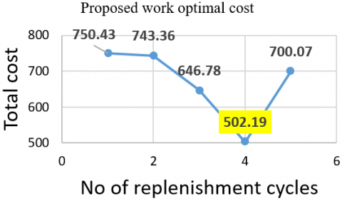
502.19 |
Figure 4. Graphic representation of sarkar model 2012
Figure 5. Proposed graphic representation
Further, Table 6, Figure 4, Figure 5 provide a comparison between proposed and existing model [18]. Moreover, it reveals that this supply chain inventory model can help the manufacturing or retail industries to reduce costs by optimizing inventory levels, and optimising replenishment time, while optimizing replenishment cycles to remain the same. Reduced costs ultimately lead to an increase in the profits.
The focus of the study is on a supply chain inventory system that deals with goods that deteriorate at a constant rate. This system includes practical and realistic characteristics that are often associated with various inventory types for a manufacturing company or retail company. The first kind, deterioration over time is a natural characteristic of anything. Second, inventory shortages are a natural phenomenon in real-world circumstances. Third, it has been discovered carbon emission cost that put an impact on the overall system cost.
Moreover, the study highlights the impact of carbon emission costs on the overall system cost. The proposed approach is particularly relevant to the retail industry or manufacturing industry. It may be utilized for metals, organic biomaterials, household items, and other things that have the preceding features.
The study provides an analytical framework for addressing the aforementioned issue and presents an optimal solution approach for determining the optimal replenishment strategy and total cost. The findings reveal that the carbon dioxide emissions significantly impact the total cost of the system. Additionally, the study examines the sensitivity of the solution to variations in various parameter values.
5.1 Managerial suggestions and future extension
The management has the flexibility to determine the optimal timing for replenishment and to halt the ordering process. Upon cessation of replenishment or ordering, the customer's demands are met by utilizing the existing inventory. The management has an understanding of the ideal moment, denoted as T, at which the inventory level will reach zero and the order should be placed to avoid stockouts.
There is potential for further expansion of this model by incorporating an inventory system with alternative carbon emission policies. Additionally, the degradation rate of the Weibull distribution may be taken into account. The cost of the manufacturing process, transportation, and refrigeration could also be considered. This model can be easily modified to account for lead time uncertainties.
[1] Noh, J., Kim, J.S. (2019). Cooperative green supply chain management with greenhouse gas emissions and fuzzy demand. Journal of Cleaner Production, 208: 1421-1435. https://doi.org/10.1016/j.jclepro.2018.10.124
[2] Toptal, A., Özlü, H., Konur, D. (2014). Joint decisions on inventory replenishment and emission reduction investment under different emission regulations. International Journal of Production Research, 52(1): 243-269. https://doi.org/10.1080/00207543.2013.836615
[3] Mishra, U., Wu, J.Z., Sarkar, B. (2021). Optimum sustainable inventory management with backorder and deterioration under controllable carbon emissions. Journal of Cleaner Production, 279: 123699. https://doi.org/10.1016/j.jclepro.2020.123699
[4] Chen, X., Benjaafar, S., Elomri, A. (2013). The carbon-constrained EOQ. Operations Research Letters, 41(2): 172-179. https://doi.org/10.1016/j.orl.2012.12.003
[5] Dye, C.Y., Yang, C.T., (2015). Sustainable trade credit and replenishment decisions with credit-linked demand under carbon emission constraints. European Journal of Operational Research, 244: 187-200. https://doi.org/10.1016/j.ejor.2015.01.026
[6] He, P., Zhang, W., Xu, X., Bian, Y., (2015). Production lot-sizing and carbon emissions under cap-and-trade and carbon tax regulations. Journal of Cleaner Production, 103: 241-248. https://doi.org/10.1016/j.jclepro.2014.08.102
[7] Xu, C., Liu, X., Wu, C., Yuan, B. (2020). Optimal inventory control strategies for deteriorating items with a general time-varying demand under carbon emission regulations. Energies, 13(4): 999. https://doi.org/10.3390/en13040999
[8] Rout, C., Paul, A., Kumar, R.S., Chakraborty, D., Goswami, A. (2020). The cooperative sustainable supply chain for deteriorating items and imperfect production under different carbon emission regulations. Journal of Cleaner Production, 272: 122170. https://doi.org/10.1016/j.jclepro.2020.122170
[9] Shi, Y., Zhang, Z., Tiwari, S., Tao, Z. (2021). Retailer's optimal strategy for a perishable product with increasing demand under various payment schemes. Annals of Operations Research: 1-31. https://doi.org/10.1007/s10479-021-04074-4
[10] Shen, Y., Shen, K., Yang, C. (2019). A production inventory model for deteriorating items with collaborative preservation technology investment under carbon tax. Sustainability, 11(18): 5027. https://doi.org/10.3390/su11185027
[11] Tiwari, S., Daryanto, Y., Wee, H.M. (2018). Sustainable inventory management with deteriorating and imperfect quality items considering carbon emission. Journal of Cleaner Production, 192: 281-292. https://doi.org/10.1016/j.jclepro.2018.04.261
[12] Gu, J.D. (2003). Microbiological deterioration and degradation of synthetic polymeric materials: Recent research advances. International Biodeterioration & Biodegradation, 52(2): 69-91. https://doi.org/10.1016/S0964-8305(02)00177-4
[13] Abad, P.L. (1996). Optimal pricing and lot-sizing under conditions of perishability and partial backordering. Management Science, 42(8): 1093-1104. https://doi.org/10.1287/mnsc.42.8.1093
[14] Deb, M., Chaudhuri, K. (1987). A note on the heuristic for replenishment of trended inventories considering shortages. Journal of the Operational Research Society, 38(5): 459-463. https://doi.org/10.1057/jors.1987.75
[15] Goyal, S.K., Morin, D., Nebebe, F. (1992). The finite horizon trended inventory replenishment problem with shortages. Journal of the Operational Research Society, 43(12): 1173-1178. https://doi.org/10.1057/jors.1992.183
[16] Giri, B.C., Chakrabarty, T., Chaudhuri, K.S. (2000). A note on a lot sizing heuristic for deteriorating items with time-varying demands and shortages. Computers & Operations Research, 27(6): 495-505. https://doi.org/10.1016/S0305-0548(99)00013-1
[17] Chakrabarti, T., Chaudhuri, K.S. (1997). An EOQ model for deteriorating items with a linear trend in demand and shortages in all cycles. International Production Economics, 49: 205-213. https://doi.org/10.1016/S0925-5273(96)00015-1
[18] Sarkar, T., Ghosh, S.K., Chaudhuri, K. (2012). An optimal inventory replenishment policy for a deteriorating item with time-quadratic demand and time-dependent partial backlogging with shortages in all cycles. Applied Mathematics and Computation, 218(18): 9147-9155. https://doi.org/10.1016/j.amc.2012.02.072
[19] Singh, P., Mishra, N.K., Singh, V., Saxena, S. (2017). An EOQ model of time quadratic and inventory-dependent demand for deteriorated items with partially backlogged shortages under trade credit. In AIP conference proceedings, 1860(1): 020037. https://doi.org/10.1063/1.4990336
[20] Khanra, S., Chaudhuri, K.S. (2003). A note on an order-level inventory model for a deteriorating item with time-dependent quadratic demand. Computers & Operations Research, 30(12): 1901-1916. https://doi.org/10.1016/S0305-0548(02)00113-2
[21] Ghosh, S.K., Chaudhuri, K.S. (2006). An EOQ model with a quadratic demand, time-proportional deterioration and shortages in all cycles. International Journal of Systems Science, 37(10): 663-672. https://doi.org/10.1080/00207720600568145
[22] Mishra, N.K., Ranu. (2022). A supply chain inventory model for deteriorating products with carbon emission-dependent demand, advanced payment, carbon tax and cap policy. Mathematical Modelling of Engineering Problems, 9(3): 615-627. https://doi.org/10.18280/mmep.090308