Khalil Benmouiza
© 2022 IIETA. This article is published by IIETA and is licensed under the CC BY 4.0 license (http://creativecommons.org/licenses/by/4.0/).
OPEN ACCESS
Nowadays, photovoltaic systems are more and more often connected to the electricity grid. They allow a household to produce part of its electricity in a clean way and to inject excess electricity production into the network. Higher output voltage and Maximum Power Point Tracking (MPPT) for each solar panel are attracting increased interest in photovoltaic solar systems with integrated converters coupled in series and parallel. In this paper, different PV arrays and converters architectures are tested in order to obtain maximum delivered power for the grid. The analysis of the output current, voltages, and power for each part of the grid-connected PV systems is analysis considering the parallel and series combination of PV arrays and DC/DC converters to extract useful information of such systems. Moreover, the performance comparison of each topology is elaborated in both cases; clear and cloudy skies. The obtained results show that using parallel configurations gives more power than series ones.
PY systems, grid connected, topologies, converters
Energy generation is a future problem. The energy demands of industrialized countries are rising. As they grow, emerging nations will require more energy. Fueled by fossil fuels, the majority of the world's energy supply originates from this source. The use of these sources causes greenhouse gas emissions and pollution. Overusing natural resources diminishes energy supplies for future generations [1].
Solar, wind, geothermal, hydroelectric, and biomass are examples of renewable energy. Renewables have endless resources, unlike fossil fuels. Renewable energies include a certain number of technological sectors according to the source of energy recovered, and the valuable energy obtained [2, 3].
With photovoltaic solar energy, for example, individuals who were previously simple consumers can now become electricity producers. As the current policy is not to self-consume this electricity but to insert it into the network, each installation must connect to it. However, until now the networks have been designed in such a way as to transport the electricity produced in a concentrated manner in high-power power stations and to distribute it for consumption by millions of consumers, individuals or businesses. This decentralization of production linked to renewable energies will therefore require new functionalities and induce a complexification of the system. The stakes are high because if not addressed, it could seriously hamper the development of renewable energies. Nowadays, photovoltaic systems are increasingly connected to the electricity grid [4, 5]. They allow a household to produce part of its electricity in a clean way and to inject excess electricity production into the network.
Several factors that may affect how much electricity a solar power system produces each year, including the performance and dependability of static converters that are used to link it to the grid. However, this connection can have some impacts on the electrical networks [6, 7], such as; the power flows changes, impact on the voltage, protection as well as the quality of the produced energy.
Several research have been conducted on the simulation and analysis of grid connected PV systems. Ranging from modelling problems [8-10], where authors aim is to give a full review and understanding about the step by step grid connected PV system modelling with their characteristics, to the performance analysis and soft computing [11-13] and faults detection and diagnosis [14-16]. However, few papers only are conducted to the study of the suitable configurations topologies in order to maximize the output power in such kind of systems.
Hence, our objective in this paper is the study the possible topologies for a large-scale grid-connected PV system. A comparison between series and parallel configurations of solar panels and converters to find the most cost-effective topology is achieved. A Matlab/Simulink comparison between the different topologies is viewed. The output current and voltage as well as the power from the PV systems as well as the converters is plotted. Moreover, partial shading PV systems is also discussed. The obtained results will help to get more information about the suitable installation in such kind of grid-connected PV systems.
The remainder of the paper is constructed as follows: Section 2 will be dedicated to the adopted methodology as well as the mathematical modelling of each part of the grid-connected PV system. In section 3, we will introduce the different proposed topologies for testing the suitable one for the grid-connected PV system. In section 4, the simulation results and discussion of the comparison between the grid connected PV systems topologies. The last section is devoted to the conclusions.
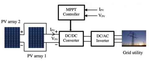
The adopted methodology consists of testing different configurations of a combination of PV panels with DC/DC converters connected to the electricity grid. The perturb and observe MPPT algorithm is used for controlling the duty cycle of the DC/DC converters. The basic Simulink model is given in Figure 1.
Figure 1. Basic Simulink model for grid connected PV system
2.1 Grid connected PV systems modelling
2.1.1 PV panels
PV panels are devices that convert light into electricity using semi-conductors. The equivalent electrical circuit of PV cell with two diodes is given in Figure 2 [17].
Figure 2. Equivalent two-diode circuit model for a PV cell
The mathematical modelling of PV panels is given in detail in several papers. Hence, we will briefly give the final mathematical model as expressed in Eq. (1).
$I=I_l-I_{d 1}\left(e^{\frac{q\left(V+I R_s\right)}{n_1 K T}}-1\right)-I_{d 2}\left(e^{\frac{q\left(V+I R_s\right)}{n_2 K T}}-1\right)$$-\frac{\left(V+I R_s\right)}{R_{S H}}$ (1)
where, $I_l$ is illumination; $T$ is the cell temperature in Kelvin, $R_S$ and $R_{S H}$ are series and shunt resistances, respectively. $V$ is the measured voltage and $K$ is constant equals $1.38 \times 10-23 \mathrm{~J} / \mathrm{K}$.
2.1.2 DC/DC converters
The DC converter transforms a DC battery voltage (12V, 24V or 48V) into a different DC voltage. Its main role is to push the PV system to get the maximum power to deliver to the grid utility using MPPT method. Two types of DC/DC converters exist, which are the buck and boost [18].
a) Buck converter
Figure 3 shows the buck DC-DC converter. If the switch is turned on, the load is connected to the power source. When the switch is turned off, no electricity flows through the device being powered [8, 9].
Figure 3. Buck converter
The duty cycle D is expressed by Eq. (2)
$D=\frac{U_E}{U_A}$ (2)
b) Boost converter
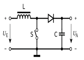
Figure 4 illustrates a boost converter, which boosts an input DC voltage to a higher DC voltage [18, 19].
Figure 4. Boost converter
The duty cycle of boost converter is calculated using by Eq. (3).
$\frac{U_A}{U_E}=\frac{1}{1-D}$ (3)
2.1.3 Maximum Power Point Tracking (MPPT)
MPPT is an algorithm that extracts the maximum generated power from a PV array. As a result, the power provided will vary depending on the load for the same illumination. In this way, an MPPT controller allows the converter to always send the greatest amount of power to the load. There are a variety of ways to implement the MPPT search algorithm depending on the implementation and performance desired. The DC/DC converter duty cycle must be varied in order for any high-performance method to work [20]. In our paper, we have used the basic MPPT algorithm, namely the perturb and observe. The summary of this algorithm is given in Figure 5.
Figure 5. Perturb and observe MPPT algorithm flowchart
2.1.4 Power system modelling
Three-phase network 3 sinusoidal quantities of the same frequency, phase between them of $2\pi/3$ (represent the 120 degree phase shift mathematically), and having even effective value, form a balanced three-phase system has been used. Choosing a 3-phase network when designing power system modeling is a common approach because it allows for a more efficient and balanced distribution of power.
The electrical distribution network is based on a three-phase system of voltages. Generally, we consider that $\left(V_a V_b V_c\right)$ is a directly balanced three-phase voltage system. It is the same for $\left(U_{a b} U_{b c} U_{c a}\right)$ as expressed in Eq. (4) and (5).
$\left\{\begin{array}{c}V_a=V_m \sin (w t) \\ V_b=V_m \sin \left(w t-\frac{2 \pi}{3}\right) \\ V_c=V_m \sin \left(w t-\frac{4 \pi}{3}\right)\end{array}\right.$ (4)
$\left\{\begin{array}{l}U_{a b}=V_a-V_b \\ U_{b c}=V_b-V_c \\ U_{c a}=V_c-V_a\end{array}\right.$ (5)
Relationships for a balanced three-phase system are given by Eq. (6);
$\left\{\begin{array}{c}V_m=\sqrt{2} V_{e f f} \\ U_m=\sqrt{3} V_m \\ U_{e f f}=\sqrt{3} V_{e f f}\end{array}\right.$ (6)
Our aim is to test different topologies to extract the maximum power with the lowest pricing. Hence, we have used 4 configurations between PV arrays and DC/DC converters as shown in Figure 6.
For topology N°1 we have connected two PV arrays with one boost converter, the output from the boost will feed the electricity grid. Topology N°2 consists of separate series combination of two PV arrays with two boost converters. In topology N° 3, we have reversed the combination by using two panels in parallel with one boost converter, and for topology N°4 we have used separate combination for one array with one boost converter in parallel with another PV array with one boost converter.
(a)
(b)
(c)
(d)
Figure 6. Different topologies: a (two array in series with one boost), b (separate series array with boost), c (two arrays in parallel with one boost), d (one array with one boost in parallel with another array with one boost)
Our objective is to test the generated power for grid-connected PV systems using different panels and DC/DC converters topologies. The simulation is conducted using MATLAB /Simulink software. A comparison between the four used topologies in both clear and partially cloudy skies is elaborated in order to judge the best topology for such cases. In what follows, we will give the used components for simulation purpose.
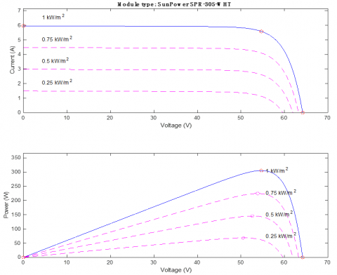
In the first place, we employed two PV arrays, each with 66 parallel strings and five series-connected modules per string. One panel is shown in Figure 7 with its I-V and P-V characteristics. In this figure, we have plotted the characteristics for different irradiation values.
Figure 7. I-V and P-V characteristics of SunPower SPR-305 WHT panel
The Module specifications under STC [ Voc, Isc, Vmp, Imp] are [ 64.2v, 5.96A, 54.7v, 5.58A], respectively. The model parameters for one module [ Rs, Rp, Isat, Iph, Qd] are [ 0.037998 Ω, 993.51 Ω, 1.1753e-08 A, 5.6902 A, 1.3], respectively.
In addition, we have used a boost converter, where the duty cycle is generated using the Perturb and observe MPPT model. The main objective is to ensure a DC bus voltage (V) equals 500 V for any topology and irradiation conditions.
VSCs are used to convert DC voltages to AC ones. It utilizes a VSC average model to transform 500 volts direct current into 260 volts alternating current. Boost and VSC converters are represented as equivalent voltage sources in the average model, which averages AC voltage across one switching frequency cycle. This model does not include harmonics, but it does maintain the dynamics of the control system's interaction with the power supply. Larger time steps (50 us) are available in this model, allowing for faster simulation. To this end, a PI controller is elaborated to guarantee this conversion. The used parameters for the VSC controller is given in Table 1.
Table 1. parameters of the VSC controller.
|
Parameters |
value |
|
Nominal power and frequency [ Pnom(VA) Fnom(Hz) ] |
[ 200e3 60] |
|
Nominal primary and secondary voltages [ Vnom_prim Vnom_sec] |
[ 25e3 260] |
|
Nominal DC bus voltage (V) |
500 |
|
Total transformer leakage impedance (pu/Pnom) [ Rxfo Lxf ] |
[0.002 0.06] |
|
Choke impedance [ R(ohm) L(H)] |
[1e-3 125e-6] |
|
VDC regultator gains [ Kp Ki] |
[7 800] |
|
Current regulator gains [ Kp Ki] |
[0.3 20] |
After that, a three-phase coupling transformer (400-kVA 260V/25kV) is used to feed the utility grid, which consists of a120-kV-equivalent transmission system with 25-kV distribution feeders as given in Figure 8.
Figure 8. Block diagram of the used utility grid.
In what follows, we will see the comparison results between different topologies.
Case 1 without shading
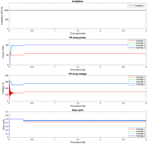
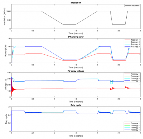
In this part, constant irradiation equal to 1000 w/m2 is used. In addition, Figure 9 shows the response from the PV array for the output power and voltage as well as the duty cycle.
We can see here that topologies N° 2, 3, and 4 give a constant power value equal to 100 kW with an output voltage of 300 V. However, for topology 1 (2 series panels with 1 boost) gives the half amount of power and voltage. This is due to the series connection, which increase the current and not voltages. Besides, we can see almost the same duty cycle but with some fluctuations, which are due to the MPPT algorithm.
Figure 10 shows the DC/DC boost output power, current, and voltages. All four topologies give a constant DC output voltage, which equals 500 V indicating the well-functioning of the MPPT method. However, we can see clearly that both topologies N° 3 and 4 give the highest amounts for output power as well as the output current. Parallel PV arrays are always favorable since they give the highest output power. However, in this case the boost converters should be also in parallel and not in series since they will not deliver the maximum DC power.
Figure 9. Solar irradiation, output PV power and voltage and duty cycle without shading
Figure 10. DC/DC converter output power, current and voltage without shading
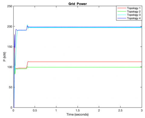
In addition, comparing the grid used power, we can see a confirmation of the above-mentioned results. As shown in Figure 11, topologies N° 3 and 4 gives the best results. The difference is in the response time and some fluctuations, which is due to the used perturb and observe tracking algorithm. Table 2 give a summary of the comparison between the results of each topology.
Table 2. Output power (without shading) for different topologies N°1 (2 array in series with 1 boost ), N°2 (2 separate series array with 1 boost ), N°3 (2 arrays in parallel with 1 boost ), N°4 (1 array with 1 boost in parallel with another 1 array with 1 boost )
|
Topologies |
PV Power |
DC /DC power |
Grid power |
|
N°1 |
50KW |
100KW |
100KW |
|
N°2 |
50 kW |
100KW |
100KW |
|
N°3 |
100 kW |
200KW |
200KW |
|
N°4 |
100 kW |
200KW |
200KW |
Case 2 With shading
In this case, we have used shaded PV arrays rather than using fixed solar irradiation. To this end, a scenario is given that simulated a different shading part during the simulation time as shown in Figure 12. In addition, this figure shows the PV array output power and voltages as well as the duty cycle.
The results confirm the ones obtained in case 1 without shading. Parallel configuration of panels always gives good results compared to series ones.
The only difference is the tracking when irradiation changes. Topologies N° 2 and 4 follow the variation fast than topology N°3, this is due to the use of two boost converts which give good response time. For the duty cycle, topology N°1 gives almost a fix values compared to others, which is not good in the case of irradiation variations.
Figure 11. Grid power generation in the case without shading
Figure 12. Solar irradiation, output PV power and voltage and duty cycle (case with shading)
For the boost converter outputs, which are shown in Figure 13 We can see a constant DC output voltage equals to 500V even in the variation of the irradiation for all topologies, the following of the constant voltage is good, which indicated the well-functioning of the MPPT method. For the outputs power and current, and as mentioned above, topologies 3 and 4 always give the highest amounts compared to topologies 1 and 2.
The grid output power for the case of partial shading shows that topologies N° 3 and 4 give the highest power. The following of the irradiation variation is clearly shown in Figure 14 and the obtained results confirm that the use of parallel array connections with boost converters is favourable.
Figure 13. DC/DC converter output power, current and voltage with shading
Figure 14. Grid power generation in the case with shading
This paper presented a comparison study between different PV grid-connected PV systems topologies. Four topologies have been tested, which vary between using two PV arrays and one or two boost converted connected in both series and parallel configurations. A comparison between the case of shading and without shading is also viewed. The obtained results show that the use of parallel connection for PV array always give better output power compared to the series connections. The same case for parallel boost converters. In addition, it is clearly shown that the DC voltage can remain constant for any kind of configuration. The use of a more advanced MPPT algorithm can reduce the fluctuations as well as the response time. However, in economic point of view, and even the use of parallel configurations gives good results, the cost can be increased significantly when using more and more arrays and DC/DC converters. Hence, a compromise between quality and cost should be taken into consideration for such systems installations and use. This analysis could take into account factors such as the expected lifespan of the system, the cost of energy, and the potential revenue or other benefits generated by the increased performance. Moreover, future works can test different topologies by varying other factors such as temperature, strong wind and light intensity.
[1] Curtin, J., McInerney, C., Ó Gallachóir, B., Hickey, C., Deane, P., Deeney, P. (2019). Quantifying stranding risk for fossil fuel assets and implications for renewable energy investment: A review of the literature. Renewable and Sustainable Energy Reviews, 116: 109402. https://doi.org/10.1016/J.RSER.2019.109402
[2] Olabi, A.G., Abdelkareem, M.A. (2022). Renewable energy and climate change. Renewable and Sustainable Energy Reviews, 158: 112111. https://doi.org/10.1016/J.RSER.2022.112111
[3] Pablo-Romero, P., Pozo-Barajas, R., Sánchez, J., García R., Holechek, J.L., Geli, H.M.E., et al. (2022). A Global Assessment: Can Renewable Energy Replace Fossil Fuels by 2050? Sustainability, 14: 4792. https://doi.org/10.3390/SU14084792
[4] Molina, M.G., Mercado, P.E. (2008). Modeling and control of grid-connected photovoltaic energy conversion system used as a dispersed generator. 2008 IEEE/PES Transmission and Distribution Conference and Exposition: Latin America, T and D-LA. https://doi.org/10.1109/TDC-LA..4641871
[5] Rani, A., Sharma, G. (2017). A Review on Grid-Connected PV System. International Journal of Trend in Scientific Research and Development, 1: 558-563. https://doi.org/10.31142/IJTSRD2195
[6] Woyte, A., Nijs, J., Belmans, R. (2003). Partial shadowing of photovoltaic arrays with different system configurations: Literature review and field test results. Solar Energy, 74: 217-233. https://doi.org/10.1016/S0038-092X(03)00155-5
[7] Wasynczuk, O. (1983). Dynamic behavior of a class of photovoltaic power systems. IEEE Transactions on Power Apparatus and Systems, 102: 3031-3037. https://doi.org/10.1109/TPAS.1983.318109
[8] Humada, A.M., Aaref A.M., Hamada H.M., Sulaiman, M.H., Amin, N., Mekhilef, S. (2018). Modeling and characterization of a grid-connected photovoltaic system under tropical climate conditions. Renewable and Sustainable Energy Reviews, 82: 2094-105. https://doi.org/10.1016/J.RSER.2017.08.053
[9] Panigrahi, S., Thakur, A. (2019). Modeling and simulation of three phases cascaded H-bridge grid-tied PV inverter. Bulletin of Electrical Engineering and Informatics, 8: 1-9. https://doi.org/10.11591/EEI.V8I1.1225
[10] Sangwongwanich, A., Yang, Y., Sera, D., Soltani, H., Blaabjerg, F. (2018). Analysis and Modeling of Interharmonics from Grid-Connected Photovoltaic Systems. IEEE Transactions on Power Electronics, 33: 8353-8364. https://doi.org/10.1109/TPEL.2017.2778025
[11] Raturi, A., Singh, A., Prasad, R.D. (2016). Grid-connected PV systems in the Pacific Island Countries. Renewable and Sustainable Energy Reviews, 58: 419-428. https://doi.org/10.1016/J.RSER.2015.12.141
[12] Anang, N., Syd Nur Azman, S.N.A., Muda, W.M.W., Dagang, A.N., Daud M.Z. (2021). Performance analysis of a grid-connected rooftop solar PV system in Kuala Terengganu. Malaysia. Energy and Buildings, 248: 111182. https://doi.org/10.1016/J.ENBUILD.2021.111182
[13] Balamurugan, M., Sahoo, S.K., Sukchai, S. (2017). Application of soft computing methods for grid connected PV system: A technological and status review. Renewable and Sustainable Energy Reviews, 75: 1493–1508. https://doi.org/10.1016/J.RSER.2016.11.210
[14] Benkercha, R., Moulahoum, S. (2018). Fault detection and diagnosis based on C4.5 decision tree algorithm for grid connected PV system. Solar Energy, 173: 610–34. https://doi.org/10.1016/J.SOLENER.2018.07.089
[15] Madeti, S.R., Singh, S.N. (2017). Online fault detection and the economic analysis of grid-connected photovoltaic systems. Energy, 134: 121–35. https://doi.org/10.1016/J.ENERGY.2017.06.005
[16] Dhimish, M., Holmes, V. (2016). Fault detection algorithm for grid-connected photovoltaic plants. Solar Energy, 137: 236–245. https://doi.org/10.1016/J.SOLENER.2016.08.021
[17] Alrahim Shannan, N.M.A., Yahaya, N.Z., Singh, B. (2013). Single-diode model and two-diode model of PV modules: A comparison. Proceedings - 2013 IEEE International Conference on Control System, Computing and Engineering, ICCSCE 2013, 210-214. https://doi.org/10.1109/ICCSCE.2013.6719960
[18] Tan, R.H.G., Hoo, L.Y.H. (2015). DC-DC converter modeling and simulation using state space approach. 2015 IEEE Conference on Energy Conversion, CENCON 2015, 42–47. https://doi.org/10.1109/CENCON.2015.7409511
[19] Gottlieb, I.M. (1994). Power supplies, switching regulators, inverters, and converters. 2nd ed. McGraw Hill Professional.
[20] Karami, N., Moubayed, N., Outbib, R. (2017). General review and classification of different MPPT Techniques. Renewable and Sustainable Energy. Reviews, 68: 1–18. https://doi.org/10.1016/J.RSER.2016.09.132