Fatima Zahra Khemili* | Moussa Lefouili | Omar Bouhali | Nassim Rizoug | Lyas Bekrar
© 2022 IIETA. This article is published by IIETA and is licensed under the CC BY 4.0 license (http://creativecommons.org/licenses/by/4.0/).
OPEN ACCESS
This work suggests a dual three-phase Space Vector Modulation (SVM) for the Diode Clamped Multilevel Inverter (DCMI) to ensure a robust control of Dual Star Induction Motor (DSIM). The principal scheme is investigated to apply the same control of the six-phase multilevel inverter by two three-phase multilevel inverter to drive the DSIM. The use of classic SVM control offers significant simplifications for controlling a six phase five levels inverter. The proposed control approach employs according to the hybridization of various conversion functions to establish the modulation strategy for each voltage vector and its placement in the plane of voltage modulation in distinctly and easy manner. A numerical simulation under MATLAB/Simulink is carried out to evaluate the Indirect Field Oriented Control (IFOC) of DSIM drive fed by multilevel inverters. The simulation outcomes clearly reveal good performance of the designed control strategy in terms of THD and control efficiency.
DSIM, IFOC, six-phase multilevel inverter, SVM
Many studies performed on analysis and modeling of multi-phase motor drive generated by multilevel converter have been realized because of their principal advantage [1]. Especially, the Dual Star Induction Motor (DSIM) is characterized by the segmented total power, low transistor current, low torque ripple at high frequency and the low rate THD of rotor currents [2-4]. Several strategies have been developed to control the DSIM amid them the Direct Toque Control (DTC), the Field Oriented Control (FOC) and the Indirect Field Oriented Control (IFOC).
The IFOC development led to a rising in the domain of elevated efficacy of drives [5], that ensure the decoupling between the torque and flux for making the motor similar to independently excited DC motor [6]. To achieve the decoupled nature of the flux and the torque, researchers have proposed (DTC) strategy. It offers a good dynamic performance with flux and torque ripples, and it reduces the ripple Discrete Space Vector Modulation (DSVM) [7].
The employment of IFOC with SVM is done to diminish the flux and torque ripples and to fix the switching frequency [8]. From several studies developed for PWM in multiphase multilevel application [9, 10], it is clear that this technique has become the most popular choice of multilevel inverter in high power application. Their main advantages are: high power rating and low harmonics rate [11-13].
Many works are performed by combining the DSIM controlled by different control strategies with the multilevel converter which is piloted by the PWM, among them; A novel design of space vector pulse width modulation (SVPWM) strategy is proposed by Kumar et al. [14] based on the fundamental reverse mapping inverters to drive the multilevel switches. A novel DTC-SVM scheme for a DSIM fed by two 3-level inverters with NPC structure presented in the study of Sadouni [15]. An advanced control scheme using new fuzzy scheme to control a DSIM supplied by two 5-level voltage source PWM inverters used in association with indirect field oriented control is proposed in the study of Bentouhamia et al. [11].
Nowadays, the Fuzzy Logic Control (FLC) has been attracting great research interests specially the type-2 fuzzy logic controller that is one of most useful control techniques to adjust the speed stabilization [16]. The authors [17] present the modeling and design of a robust neuro-fuzzy inference strategy (ANFIS) for ensuring the control of the DSIM speed supplied by three-phase direct matrix converter via SVM.
In the study of Lyas et al. [18], an effective dual three-phase SVM for six phase multilevel inverter is suggested to achieve a robust driving of six-phase induction machine (SPIM) by controlling the six-phase multilevel inverter as two three phase induction drive (1, 3 and 5) phase with the first star and (2, 4 and 6) phase with the second star, by using the three-phase Separate DC Source (SDCS) inverter controlled by N level SVM. In this paper, we changed the six-phase SDCS by two three-phase DCI as mentioned in the study of Lyas et al. [18].
The paper presents a combination of the modulation techniques of the 5-level single-phase DCI and the 3-level three-phase DCI in order to control the modulation method for a three-phase five-level DCI. The principal idea of this system is inspired from a general modulation.
A supplementary suitable design and modeling for the system conception is performed according to a direct space vector control of line-to-line voltages. Usually, the SVM frame is decomposed into triangular regions in which the three vectors are employed to generate the PWM waveform, and it is fastened with the region that contains the vector reference. Consequently, In SVM scheme control, all switching modulation values can be exhibited by attaining 61 diverse scheme structures, that are denoted by ux(i,j) in the frame (0,um1/us1/4,um2/us1/4) [19].
In this research, the 61 voltage vectors of the 5-level inverter are employed for the modulation control. The redundant vectors can be anticipated for the DC bus voltage balancing as in the study of Bouhali et al. [20]. The simulations results of the IFOC of DSIM fed by a Dual DCI and controlled by the SVM show the high performance and great efficiency of the proposed modulation technique.
This work is organized as follows; Section (2) presents the modeling of DSIM. In the section (3), we explain the multilevel inverter operating principle and the converter modeling. Section (4) shows the implementation of the proposed control strategies. Final section offers the obtained result.
The DSIM contains of a mobile rotor winding along with two fixed three-phase stator windings oriented with an electrical angle $\alpha$.
where, (As1, Bs1, Cs1) are the wending of the first star and (As2, Bs2, Cs2) are the wending of the second one, α is the angle between them and is equal 30o. (Ar, Br, Cr) are the wending of rotor of DSIM, which are sinsoidally distributed, and they have the axes displaced apart by 120 degree [21]. Figure 1 shows schematically the windings of the DSIM.
Figure 1. Winding’s scheme of DSIM
2.1 The electrical equations
In matrix form, the equations of DSIM model in park frame are given by [22]:
$\left\{\begin{array}{l}\left.\left[v_{s 1}\right]=\left[R_{s 1}\right] [I_{S 1}\right]+\frac{d}{d t}\left[\psi_{s 1}\right] \\ \left.\left[v_{s 2}\right]=\left[R_{s 2}\right] [I_{S 2}\right]+\frac{d}{d t}\left[\psi_{s 2}\right] \\ {\left[v_r\right]=\left[R_r\right]\left[I_r\right]+\frac{d}{d t}\left[\psi_r\right]}\end{array}\right.$ (1)
with, $\left[\psi_{s 1}\right]=\left[\psi_{a s 1} \,\, \psi_{b s 1} \,\, \psi_{c s 1}\right]^T,\left[v_{s 1}\right]=\left[v_{a s 1} \,\, v_{b s 1} \,\, v_{c s 1}\right]^{T}$and $\left[I_{s 1}\right]=\left[i_{a s 1} \,\, i_{b s 1} \,\, i_{c s 1}\right]^T$.
$\left[ R _{ s 1}\right]=\left[\begin{array}{ccc} R _{ as 1} & 0 & 0 \\ 0 & R _{b s 1} & 0 \\ 0 & 0 & R _{ cs1 }\end{array}\right],\left[ R _{ s 2}\right]=\left[\begin{array}{ccc} R _{ as 2} & 0 & 0 \\ 0 & R _{b s 2} & 0 \\ 0 & 0 & R _{ cs 2}\end{array}\right]$
$\left[R_r\right]=\left[\begin{array}{ccc}R_{a r} & 0 & 0 \\ 0 & R_{b r} & 0 \\ 0 & 0 & R_{c r}\end{array}\right]$
2.2 Magnetic equations
The flux expressions are given by [22]:
$\left[\begin{array}{l}{\left[\psi_{a b c, s 1}\right]} \\ {\left[\psi_{a b c, s 2}\right]} \\ {\left[\psi_{a b c, r}\right]}\end{array}\right]=\left[\begin{array}{ccc} \left[L_{s 1 s 1}\right] & {\left[l_{s 1 s 2}\right]} & {\left[l_{s 1 r}\right]} \\ \left[l_{s 2 s 1}\right] & {\left[l_{s 2 s 2}\right]} & {\left[l_{s 2 r}\right]} \\ \left[ l_{r s 1}\right] & {\left[l_{r s 2}\right]} & {\left[l_{r r}\right]}\end{array}\right]$ (2)
with the inductance matrix are:
$\left[L_{s 1, s 1}\right]=\left[\begin{array}{ccc}\left(L_{a s 1}+L_{m s}\right) & -L_{m s} / 2 & -L_{m s} / 2 \\ -L_{m s} / 2 & \left(L_{b s 1}+L_{m s}\right) & -L_{m s} / 2 \\ -L_{m s} / 2 & -L_{m s} / 2 & \left(L_{c s 1}+L_{m s}\right)\end{array}\right]$
$\left[L_{s 2, s 2}\right]=\left[\begin{array}{ccc}\left(L_{a s 2}+L_{m s}\right) & -L_{m s} / 2 & -L_{m s} / 2 \\ -L_{m s} / 2 & \left(L_{b s 2}+L_{m s}\right) & -L_{m s} / 2 \\ -L_{m s} / 2 & -L_{m s} / 2 & \left(L_{c s 2}+L_{m s}\right)\end{array}\right]$
$\left[L_{r, r}\right]=\left[\begin{array}{ccc}\left(L_{a r}+L_{m r}\right) & -L_{m r} / 2 & -L_{m r} / 2 \\ -L_{m r} / 2 & \left(L_{b r}+L_{m r}\right) & -L_{m r} / 2 \\ -L_{m r} / 2 & -L_{m r} / 2 & \left(L_{c r}+L_{m r}\right)\end{array}\right]$
To facilitate the differential equations, the park transformation consists in transforming the three-phase stator (and rotor) windings system of axes a, b and c into a system equivalent with two-phase windings of axis (d,q) by creating the same magnetic force. Park matrix is given as:
$[p(\theta)]=\sqrt{\frac{2}{3}}\left[\begin{array}{ccc}\cos \cos (\theta) & \cos \cos \left(\theta-\frac{2 \pi}{3}\right) & \cos \cos \left(\theta+\frac{2 \pi}{3}\right) \\ -\sin -\sin (\theta) & -\sin \left(\theta--\sin \left(\theta-\frac{2 \pi}{3}\right)\right. & -\sin \left(\theta+-\sin \left(\theta+\frac{2 \pi}{3}\right)\right. \\ \frac{1}{2} & \frac{1}{2} & \frac{1}{2}\end{array}\right]$
$X_{(d q 0) i}=[p(\theta)]^{-1} X_{(\alpha \beta 0) i}$ (3)
where, X denote the voltage, the current, or the flux and i can take 1 and 2 which indicates the first stator and the second stator. The DSIM equations in the synchronous reference frame (d, q) are expressed by following:
$\left\{\begin{array}{l}v_{d s 1}=R_s i_{d s 1}+\frac{d}{d t} \psi_{d s 1}-w_{c o o r} \psi_{q s 1} \\ v_{q s 1}=R_s i_{q s 1}+\frac{d}{d t} \psi_{q s 1}+w_{c o o r} \psi_{d s 1} \\ v_{d s 2}=R_s i_{d s 2}+\frac{d}{d t} \psi_{d s 2}-w_{c o o r} \psi_{q s 2} \\ v_{q s 2}=R_s i_{q s 2}+\frac{d}{d t} \psi_{q s 2}+w_{c o o r} \psi_{d s 2} \\ v_{d r}=R_r i_{d r}+\frac{d}{d t} \psi_{d r}-\left(w_{c o o r}-w_r\right) \psi_{q r}=0 \\ v_{q r}=R_r i_{q r}+\frac{d}{d t} \psi_{q r}+\left(w_{c o o r}-w_r\right) \psi_{d r}=0\end{array}\right.$ (4)
with, wcoor is an angular speed of the axes (d, q). The dual stator and the rotor flux expressions are [23]:
$\left\{\begin{array}{l}\psi_{d s 1}=L_{s 1} i_{d s 1}+L_m\left(i_{d s 1}+i_{d s 2}+i_{d r}\right) \\ \psi_{q s 1}=L_{s 1} i_{q s 1}+L_m\left(i_{q s 1}+i_{q s 2}+i_{q r}\right) \\ \psi_{d s 2}=L_{s 2} i_{d s 2}+L_m\left(i_{d s 1}+i_{d s 2}+i_{d r}\right) \\ \psi_{q s 2}=L_{s 2} i_{q s 2}+L_m\left(i_{q s 1}+i_{q s 2}+i_{q r}\right) \\ \psi_{d r}=L_r i_{d r}+L_m\left(i_{d r}+i_{d s 1}+i_{d s 2}\right) \\ \psi_{q r}=L_r i_{q r}+L_m\left(i_{q r}+i_{q s 1}+i_{q s 2}\right)\end{array}\right.$ (5)
where, Lm is cyclic mutual inductance between star 1 and 2 and the rotor, with $\frac{3}{2} L_{m s}=\frac{3}{2} M_{s r}=\frac{3}{2} L_{m r}=L_m$.
The form of state equation or the system related to the rotating field are mentioned below. It is mentioning that with wcoor=ws:
$\left\{\begin{array}{l}\frac{d}{d t} \psi_{d s 1}=v_{d s 1}-R_{s 1} i_{d s 1}+w_s \psi_{q s 1} \\ \frac{d}{d t} \psi_{q s 1}=v_{q s 1}-R_{s 1} i_{q s 1}-w_s \psi_{d s 1} \\ \frac{d}{d t} \psi_{d s 2}=v_{d s 2}-R_{s 2} i_{d s 2}+w_s \psi_{q s 2} \\ \frac{d}{d t} \psi_{q s 2}=v_{q s 2}-R_{s 2} i_{q s 2}-w_s \psi_{d s 2} \\ \frac{d}{d t} \psi_{d r}=v_{d r}-R_r i_{d r}+\left(w_s-w_r\right) \psi_{q r}=0 \\ \frac{d}{d t} \psi_{q r}=v_{q r}-R_r i_{q r}-\left(w_s-w_r\right) \psi_{d r}=0\end{array}\right.$ (6)
where, vdqs1 and vdqs2 are the stator voltages. $i_{d q s 1}$ and $i_{d q s 2}$ components are the stator current. vdqr and idqr components are the rotor voltage and current. $\psi_{d q s 1}$, $\psi_{d q s 2 r}$ and $\psi_{d q r}$ components are the stator and the rotor flux components. ws denotes the synchronous reference speed. wr represents the rotor electrical angular speed. Rs1, Rs2 and Rr mean the stator and rotor resistance respectively.
It is possible to obtain the other expressions of the torque by using the expressions of the stator flows and by replacing them in Eq. (5):
$C_{e m}=P L_m\left[\left(i_{q s 1}+i_{q s 2}\right) i_{d r}-\left(i_{d s 1}+i_{d s 2}\right) i_{q r}\right]$ (7)
By putting the equation system as a system of state equations, we can obtain:
$\dot{X}=A X+B U$
where, $\left\{\begin{array}{c} X=\left[\psi_{d s 1} \,\, \psi_{d s 2} \,\, \psi_{q s 1} \,\, \psi_{q s 2} \,\, \psi_{d r} \,\, \psi_{q r}\right]^T ; \text { is the state vector. } \\ U=\left[v_{d s 1} \,\, v_{d s 2} \,\, v_{q s 1} \,\, v_{q s 2}\right]^T ; \text { is the command vector. }\end{array}\right.$
where,
$A=\left[\begin{array}{cccccc} -\left( \frac{{{\text{R}}_{\text{s}1}}}{{{\text{L}}_{\text{s}1}}}-\frac{{{\text{R}}_{\text{s}1}}{{\text{L}}_{\text{a}}}}{\text{L}_{\text{s}1}^{2}} \right) & \frac{{{\text{R}}_{\text{s}1}}{{\text{L}}_{\text{a}}}}{{{\text{L}}_{\text{s}1}}{{\text{L}}_{\text{s}2}}} & {w}_{s} & 0 & \frac{{{\text{R}}_{\text{s}1}}{{\text{L}}_{\text{a}}}}{{{\text{L}}_{s1}}{{L}_{_{r}}}} & 0 \\ \frac{{{\text{R}}_{\text{s}2}}{{\text{L}}_{\text{a}}}}{{{\text{L}}_{\text{s}1}}{{\text{L}}_{\text{s}2}}} & -\left( \frac{{{\text{R}}_{\text{s}2}}}{{{\text{L}}_{\text{s}2}}}-\frac{{{\text{R}}_{\text{s}2}}{{\text{L}}_{\text{a}}}}{\text{L}_{\text{s}2}^{2}} \right) & 0 & {{\text{w}}_{\text{s}}} & \frac{{{\text{R}}_{S2}}{{\text{L}}_{\text{a}}}}{{{\text{L}}_{S2}}{{L}_{_{r}}}} & 0 \\ -{{\text{w}}_{\text{s}}} & 0 & -\left( \frac{{{\text{R}}_{\text{s}1}}}{{{\text{L}}_{\text{s}1}}}-\frac{{{\text{R}}_{\text{s}1}}{{\text{L}}_{\text{a}}}}{\text{L}_{\text{s}1}^{2}} \right) & \frac{{{\text{R}}_{\text{s}1}}{{\text{L}}_{\text{a}}}}{{{\text{L}}_{\text{s}1}}{{\text{L}}_{\text{s}2}}} & 0 & \frac{{{\text{R}}_{\text{s}1}}{{\text{L}}_{\text{a}}}}{{{\text{L}}_{s1}}{{L}_{_{r}}}} \\ 0 & -{{\text{w}}_{\text{s}}} & \frac{{{\text{R}}_{\text{s}2}}{{\text{L}}_{\text{a}}}}{{{\text{L}}_{\text{s}1}}{{\text{L}}_{\text{s}2}}} & \left( \frac{{{\text{R}}_{\text{s}2}}}{{{\text{L}}_{\text{s}2}}}-\frac{{{\text{R}}_{\text{s}2}}{{\text{L}}_{\text{a}}}}{\text{L}_{\text{s}2}^{2}} \right) & 0 & \frac{{{\text{R}}_{S2}}{{\text{L}}_{\text{a}}}}{{{\text{L}}_{S2}}{{L}_{_{r}}}} \\ \frac{{{\text{R}}_{\text{r}}}{{\text{L}}_{\text{a}}}}{{{\text{L}}_{\text{s}1}}{{\text{L}}_{\text{r}}}} & \frac{{{\text{R}}_{\text{r}}}{{\text{L}}_{\text{a}}}}{{{\text{L}}_{\text{r}}}{{\text{L}}_{\text{s}2}}} & 0 & 0 & -\left( \frac{{{\text{R}}_{r}}}{{{\text{L}}_{r}}}-\frac{{{\text{R}}_{r}}{{\text{L}}_{\text{a}}}}{\text{L}_{r}^{2}} \right) & ({{w}_{s}}\,-w\,) \\ 0 & 0 & \frac{{{\text{R}}_{\text{r}}}{{\text{L}}_{\text{a}}}}{{{\text{L}}_{\text{S}1}}{{\text{L}}_{\text{r}}}} & \frac{{{\text{R}}_{\text{r}}}{{\text{L}}_{\text{a}}}}{{{\text{L}}_{\text{r}}}{{\text{L}}_{\text{s}2}}} & ({{w}_{s}}\,-w\,) & -\left( \frac{{{\text{R}}_{r}}}{{{\text{L}}_{r}}}-\frac{{{\text{R}}_{r}}{{\text{L}}_{\text{a}}}}{\text{L}_{r}^{2}} \right) \end{array}\right]$
$B=\left[ \begin{array}{cccccc} 1\,\,\,\,\,\,0\,\,\,\,\,0\,\,\,\,\,0 \\ 0\,\,\,\,\,1\,\,\,\,\,\,0\,\,\,\,\,0 \\ 0\,\,\,\,\,0\,\,\,\,\,1\,\,\,\,\,\,0 \\ 0\,\,\,\,\,0\,\,\,\,\,0\,\,\,\,\,1 \\0\,\,\,\,\,0\,\,\,\,\,0\,\,\,\,\,0 \\ 0\,\,\,\,\,0\,\,\,\,\,0\,\,\,\,\,0 \\ \end{array} \right]$
3.1 Structure and operating principle
The main scheme structure of a 5-level three-phase DCI involves three commutation circuits, which are fed by four capacitors that can attain practically the similar voltage level (us1/4). The converter can employ under the operation of PWM mode. Figure 2 illustrates the schematic configuration of DCI [20].
Figure 2. Schematic structure of a 5-level three-phase
3.2 DCI principle
The equivalence representation of matrix structure of the five-level DCI indicates that for each commutation circuit (c) c ϵ (1,2,3) has the 5 various topology of switching function (frc) rϵ(1,2,3,4,5) as exposed in Figure 3. The clamped commutation structure is similar to a commutation structure with five ideal switches. The switch states are named switching functions (frc). Profoundly, if frc=1, it signifies that the matching ideal switch is closed. Contrary, in case of frc=0, the switch is open.
where, r represents the total number of the ideal matrix row while c denotes the column, $r \in\{1,2,3,4,5\}, c \in\{1,2,3\}$.
The final switching function is determined via the other ones as: $f_{5 c}=\bar{f}_{1 c} \cdot \bar{f}_{2 c} \cdot \bar{f}_{3 c} \cdot \bar{f}_{4 c}$. Five different configurations of frc exists for each commutation circuit. The mentioned topology permits easily the association of the capacitor voltage divider with the load. The equivalent circuit of commutation are tabulated in Table 1.
Figure 3. Equivalent structure of the five level DCI
In order to implement and realize the desired switching functions, the matching gate signals of transistors are attained by following:
$\left\{ \begin{align} & {{T}_{1c}}={{f}_{ref\_1c}} \,\,, \\ & {{T}_{2c}}={{f}_{ref\_1c}}+{{f}_{ref\_2c}} \,\,, \\ & {{T}_{3c}}={{f}_{ref\_1c}}+{{f}_{ref\_2c}}+{{f}_{ref\_3c}} \,\,, \\ & {{T}_{4c}}={{f}_{ref\_1c}}+{{f}_{ref\_2c}}+{{f}_{ref\_3c}}+{{f}_{ref\_4c}} \\ & {{T}_{(4+r)c}}={{{\bar{T}}}_{rc}} \,\, ,\ for\quad r\in \left\{ 1,2,3,4 \right\} \\\end{align} \right.$ (8)
Table 1. Equivalent circuit of commutation
|
|
|
T |
|
|
|
f0c |
|
|
|
T1C |
T5C |
T6C |
T7C |
T8C |
f1c |
f2c |
f5c |
uso |
|
1 |
0 |
0 |
0 |
0 |
1 |
0 |
0 |
us1 |
|
0 |
1 |
0 |
0 |
0 |
0 |
1 |
0 |
3us1/4 |
|
0 |
1 |
1 |
0 |
0 |
0 |
0 |
0 |
us1/2 |
|
0 |
1 |
1 |
1 |
0 |
0 |
0 |
0 |
us1/4 |
|
0 |
1 |
1 |
1 |
1 |
0 |
0 |
1 |
0 |
The proposed space vector control uses a simple algebra equation for determining each vector duration by using the obtained projection into frame vector. Sixty-one various structures are employed and defined by ux(i, j) in the frame (0, um1 / us1 /4, um2 / us1 /4) as shown in Figure 4.
The frame is accordingly decomposed into 184 triangular regions. The mean value of voltages modulation may be adjusted respectively by three vectors switching. This operation presents the sector in case of the suitable voltage placed. All values of switching functions can be considered by acquiring all possible modulated voltages vectors as mentioned in the study of Khemili et al. [19].
Also, in order to examine the consequence of the conversions, eight modulation functions (mrp) are utilised and exposed as follows:
${{m}_{rp}}={{f}_{rp}}-{{f}_{r3}}$ (9)
where, $r \in(1,2,3,4)$ and $p \in(1,2)$.
In this control, merely two phase-to-phase modulated voltages are considered from the equivalent structure of the five level DCI and expressed by:
$\begin{array}{} {{um}_{1}}={{v}_{10}}-{{v}_{30}}=\sum\limits_{{}}^{{}}{({{f}_{r1}}}-{{f}_{r3}})u{{s}_{r}} \\ u{{m}_{2}}={{v}_{20}}-{{v}_{30}}=\sum\limits_{{}}^{{}}{(f2}-{{f}_{r3}})u{{s}_{r}} \\ u{{m}_{3}}=u{{m}_{1}}-um2 \\ \end{array}$ (10)
As a result of this, each vector duration is mainly obtained by means of the achieved projection onto frame vector by means of four principal sectors. The sector where the positioned vector may be revealed via function (fix) and (sign). Thus, Figure 5 illustrates the graphical illustration of the function fix.
Figure 4. Space vector position into the frame
Figure 5. Graphical illustration of the function fix
$\left(0, \frac{\vec{u}_{m_1}}{u_{s_1} / 4}, \frac{\vec{u}_{m_2}}{u_{s_1} / 4}\right)$
The function y=sign(x) can be presented as:
$y=1$ if $\quad x>0$
$y=-1$ if $\quad x<0$
Initial duty cycles of modulated voltages are defined as given in the following equation:
$r_1=\frac{\left\langle u_{m 1}\right\rangle}{u s_1 / 4}, \quad r_2=\frac{\left\langle u_{m 2}\right\rangle}{u s_1 / 4}$
where, $\left\langle u _{m 1}\right\rangle$ and $\left\langle u _{m 2}\right\rangle$ present the values of modulated voltages. The sector, where the vector is placed and revealed via the function (fix) is presented by:
$y=\operatorname{fix}(x)=a$ if $x \in[a, a+\operatorname{sign}(a)[, \quad$ with $a \in Z$
This sector is achieved by means of the parameters i and j:
$i={fix}\left(r_1\right), \quad j={fix}\left(r_2\right)$
This SVM use four sectors for detected the desired voltage vector that for every sector two triplets of vector exist as exposed in Figure 6.
Figure 6. Extended observation of the generalized studied sector
For sector number 1, we get:
$\vec{u}_1=\vec{u}(i, j), \vec{u}_2=\vec{u}\left(i+\operatorname{sign}\left(r_1\right), j\right)$
and $\vec{u}_3=\vec{u}\left(i, j+\operatorname{sign}\left(r_2\right)\right)$ (11)
Or
$\vec{u}_1=\vec{u}\left(i, j+\operatorname{sign}\left(r_2\right)\right)$
$\vec{u}_2=\vec{u}\left(i+\operatorname{sign}\left(r_1\right), j+\operatorname{sign}\left(r_2\right)\right)$
and $\vec{u}_3=\vec{u}(i, j)$ (12)
For sector (2):
$\vec{u}_1=\vec{u}(i, j), \vec{u}_2=\vec{u}\left(i+\operatorname{sign}\left(r_1\right), j\right)$
and $\vec{u}_3=\vec{u}\left(i, j+\operatorname{sign}\left(r_2\right)\right)$ (13)
Or
$\vec{u}_1=\vec{u}\left(i+\operatorname{sign}\left(r_1\right), j\right), \vec{u}_2=\vec{u}(i, j)$
and $\vec{u}_3=\vec{u}\left(i+\operatorname{sign}\left(r_1\right), j+\operatorname{sign}\left(r_2\right)\right)$ (14)
For sector (3):
$\vec{u}_1=\vec{u}\left(i+\operatorname{sign}\left(r_1\right), j\right), \vec{u}_2=\vec{u}(i, j)$
and $\vec{u}_3=\vec{u}\left(i+\operatorname{sign}\left(r_1\right), j+\operatorname{sign}\left(r_2\right)\right)$. (15)
Or
$\vec{u}_1=\vec{u}\left(i+\operatorname{sig} n\left(r_1\right), j+\operatorname{sig} n\left(r_2\right)\right)$
$\vec{u}_2=\vec{u}\left(i, j+\operatorname{sign}\left(r_2\right)\right)$
and $\vec{u}_3=\vec{u}\left(i+\operatorname{sig}\left(r_1\right), j\right)$ (16)
For sector (4):
$\vec{u}_1=\vec{u}\left(i+\operatorname{sign}\left(r_1\right), j\right), \vec{u}_2=\vec{u}(i, j)$
and $\vec{u}_3=\vec{u}\left(i+\operatorname{sign}\left(r_1\right), j+\operatorname{sign}\left(r_2\right)\right)$ (17)
Or
$\vec{u}_1=\vec{u}\left(i+\operatorname{sign}\left(r_1\right), j+\operatorname{sign}\left(r_2\right)\right)$
$\vec{u}_2=\vec{u}\left(i, j+\operatorname{sign}\left(r_2\right)\right)$
and $\vec{u}_3=\vec{u}\left(i+\operatorname{sign}\left(r_1\right), j\right)$ (18)
We have selected the triplet, which produces the several redundant vectors within the hexagonal shape.
In the basic rule of the SVM, the totally different duration must be similar to the modulate period:
$\frac{\vec{u}m}{{u{{s}_{1}}}/{4}\;}=\frac{t_{1}^{{}}}{Tm}.\vec{u}_{1}^{{}}\text{ }+\frac{t_{2}^{{}}}{Tm}.\vec{u}_{2}^{{}}\text{ }+\frac{t_{3}^{{}}}{Tm}.\vec{u}_{3}^{{}}$ (19)
$t_1+t_2+t_3=t_m$ (20)
Using Eqns. (19) and (20), we get:
$\frac{{{{\vec{u}}}_{m}}}{{u{{s}_{1}}}/{4}\;}=\frac{1}{{{T}_{m}}}\left( \left( {{T}_{m}}-{{t}_{2}}-{{t}_{3}} \right).{{{\vec{u}}}_{1}}+{{t}_{2}}.{{{\vec{u}}}_{2}}+{{t}_{3}}.{{{\vec{u}}}_{3}} \right)$ (21)
$\frac{{{{\vec{u}}}_{m}}}{{u{{s}_{1}}}/{4}\;}=\frac{1}{{{T}_{m}}}\left( {{t}_{2}}.\left( {{{\vec{u}}}_{2}}-{{{\vec{u}}}_{1}} \right)+{{t}_{3}}.\left( {{{\vec{u}}}_{3}}-{{{\vec{u}}}_{1}} \right)+{{T}_{m}}.{{{\vec{u}}}_{1}} \right)$ (22)
By dividing with the small level value (us1∕4) we can get:
$\frac{{{{\vec{u}}}_{m}}}{{u{{s}_{1}}}/{4}\;}\text{ }=\text{ }\frac{\left\langle {{u}_{m1}} \right\rangle }{{u{{s}_{1}}}/{4}\;}\text{ }.\vec{x}\text{ }+\text{ }\frac{\left\langle {{u}_{m2}} \right\rangle }{{u{{s}_{1}}}/{4}\;}\text{ }.\vec{y}$ (23)
1. If the wished voltage vector is positioned in sector 1 (i.e.$\left|\left\langle u_{m 1}^*\right\rangle\right|+\left|\left\langle u_{m 2}{ }^*\right\rangle\right| \leq 1$ and $\left|\left\langle u_{m 1}{ }^*\right\rangle\right| \leq\left|u_{m 2}{ }^*\right\rangle \mid$ or sector 2 (i.e.$\left| \left\langle u_{m 1}{ }^*\right\rangle\right|+\left| \left\langle u_{m 2}{ }^*\right\rangle\right| \leq 1$ and $\left| \left\langle u_{m 1}{ }^* \right\rangle \right| \geq | \left\langle u_{m 2}{ }^* \right\rangle \mid$ the vector $\vec{u}_1=\vec{u}(i, j)$ (Eq. (11) or (12)) is selected as the corner vector in that case the voltage vector is presented through this vector by following:
$\frac{{{{\vec{u}}}_{m}}}{{u{{s}_{1}}}/{4}\;}=\vec{u}(i,j)+\left\langle {{u}_{m1}}^{*} \right\rangle \vec{x}+\left\langle {{u}_{m2}}^{*} \right\rangle \vec{y}$ (24)
with
$\vec{u}(i,j)=i.\vec{x}+j.\vec{y}$ (25)
Vectors differentials from the triplet are exposed as [20]:
$\left\{ \begin{align} & {{{\vec{u}}}_{2}}-{{{\vec{u}}}_{1}}=sign({{r}_{1}})\ \vec{x} \\ & {{{\vec{u}}}_{3}}-{{{\vec{u}}}_{1}}=sign({{r}_{2}})\ \vec{y} \\ \end{align} \right.$ (26)
By replacing this equation into (22) we get:
$\frac{{{{\vec{u}}}_{m}}}{{u{{s}_{1}}}/{4}\;}=\frac{1}{{{T}_{m}}}\left( {{t}_{2}}sign({{r}_{1}})\ \vec{x}+{{t}_{3}}sign({{r}_{2}})\ \vec{y}+{{T}_{m}}\left( i.\vec{x}+j.\vec{y} \right) \right)$ (27)
$\frac{{{{\vec{u}}}_{m}}}{{u{{s}_{1}}}/{4}\;}=\left( \frac{{{t}_{2}}}{{{T}_{m}}}sign({{r}_{1}})+i \right)\ \vec{x}+\left( \frac{{{t}_{3}}}{{{T}_{m}}}sign({{r}_{2}})+j \right)\ \vec{y}$ (28)
By using these expressions and Eq. (24), we get:
$t_2=T_m\left\langle u_{m_1}{ }^*\right\rangle \operatorname{sign}\left(r_1\right)$
${{t}_{3}}={{T}_{m}}\left\langle u{{m}_{2}}^{*} \right\rangle sign({{r}_{2}})$ (29)
Or ${{t}_{2}}={{T}_{m}}\left| \left\langle u{{m}_{1}}^{*} \right\rangle \right|$
and ${{t}_{3}}={{T}_{m}}\left| \left\langle u{{m}_{2}}^{*} \right\rangle \right|$ (30)
2. If the voltage vector is placed in sector 3 i.e.
if $\left(\left|\left\langle u_{m 1}{ }^*\right\rangle\right|+\left|\left\langle u_{m 2}{ }^*\right\rangle\right|>1\right.$ and $\left.\left|\left\langle u_{m 1}{ }^*\right\rangle\right| \leq\left|\left\langle u_{m 2}{ }^*\right\rangle\right|\right)$
The vector $\overrightarrow{u_1}=\vec{u}\left(i, j+\operatorname{sign}\left(r_2\right)\right)$ is selected (Eq. (15)) as the corner vector where the modulated voltage vectors is defined with this vector as:
$\frac{{{{\vec{u}}}_{m}}}{{u{{s}_{1}}}/{4}\;}=\vec{u}(i,j+sign({{r}_{2}}))+\left\langle {{u}_{m1}}^{*} \right\rangle \vec{x}+\left( \left\langle {{u}_{m2}}^{*} \right\rangle -sign({{r}_{2}}) \right)\vec{y}$ (31)
with
$\vec{u}(i,j+sign({{r}_{2}}))=i.\vec{x}+\left( j+sign({{r}_{2}}) \right).\vec{y}$ (32)
We get
$\frac{{{{\vec{u}}}_{m}}}{{u{{s}_{1}}}/{4}\;}=i.\vec{x}+\left( j+sign({{r}_{2}}) \right).\vec{y}+\left\langle {{u}_{m1}}^{*} \right\rangle \vec{x}+\left( \left\langle {{u}_{m2}}^{*} \right\rangle -sign({{r}_{2}}) \right)\vec{y}$ (33)
Differentials of vectors is exposed as:
$\left\{ \begin{align} & {{{\vec{u}}}_{2}}-{{{\vec{u}}}_{1}}=-sign({{r}_{1}})\ \vec{x} \\ & {{{\vec{u}}}_{3}}-{{{\vec{u}}}_{1}}=-sign({{r}_{2}})\ \vec{y} \\ \end{align} \right.$ (34)
By replacing this equation into (20) we obtain:
$\frac{{{{\vec{u}}}_{m}}}{{u{{s}_{1}}}/{4}\;}=\left( -\frac{{{t}_{2}}}{{{T}_{m}}}sign({{r}_{1}})+i \right)\ \vec{x}+\left( -\frac{{{t}_{3}}}{{{T}_{m}}}sign({{r}_{2}})+j+sign({{r}_{2}}) \right)\ \vec{y}$ (35)
After this expression time durations are easily found as:
${{t}_{2}}={{T}_{m}}\left| \left\langle u{{m}_{1}}^{*} \right\rangle \right|$ and ${{t}_{3}}={{T}_{m}}\left| \left\langle u{{m}_{2}}^{*} \right\rangle -sign({{r}_{2}}) \right|$ (36)
3. If the voltage vector is located in sector, i.e
$if\quad \left( \left| \left\langle {{u}_{m1}}^{*} \right\rangle \right|+\left| \left\langle {{u}_{m2}}^{*} \right\rangle \right|>1\ \text{and}\left| \left\langle {{u}_{m1}}^{*} \right\rangle \right|\ge \left| \left\langle {{u}_{m2}}^{*} \right\rangle \right|\, \right)$
The vector is $\overrightarrow{u_1}=\vec{u}\left(i+\operatorname{sign}\left(r_1\right), j\right)$ selected as the corner vector (Eq. (17)). Then, the modulated voltage is got as:
${{t}_{2}}={{T}_{m}}\left| \left\langle u{{m}_{1}}^{*} \right\rangle -sign({{r}_{1}}) \right|$ and ${{t}_{3}}={{T}_{m}}\left| \left\langle u{{m}_{2}}^{*} \right\rangle \right|$ (37)
The objective of indirect field-oriented control (IFOC) is to assimilate the operating mode of the asynchronous machine to DC machine with separated excitation, we can do that by decoupling the torque and flux. This decoupling will simplify the analysis and control of DSIM [24]. In case of rotor flux orientation, the flux of ''q'' component will be null (ϕqr=0) and the flux of 'd' will be the desired rotor flux $\left(\phi_{d r}=\phi_r^*\right)$. The principle field control is shown by the Figure 7, while Figure 8 presents a comprehensive speed control diagram of the DSIM by the IFOC.
By applying this principle into the system equation, the result of speed slip and electromagnetic are:
$w_{sr}^{*}=L{{R}_{S}}\left( i_{qs1}^{*}+i_{qs2}^{*} \right)/\phi _{r}^{*}$ (38)
With, the system is defined by the follow equation:
${{w}_{r}}={{w}_{s}}-w=M{{i}_{sq}}/{{T}_{r}}{{\phi }_{r}}$ (39)
$\left\{ \begin{align} & {{\phi }_{sd}}={{L}_{s}}\left( 1-\frac{{{M}^{2}}}{{{L}_{s}}{{L}_{r}}} \right){{i}_{sd}}+\frac{M}{{{L}_{r}}}\phi \\ & {{\phi }_{sq}}={{L}_{s}}\left( 1-\frac{{{M}^{2}}}{{{L}_{s}}{{L}_{r}}} \right){{i}_{sq}} \\\end{align} \right. $ (40)
$\left\{ \begin{align} & {{v}_{sd}}={{R}_{s}}{{i}_{sd}}+\sigma {{L}_{s}}\frac{d{{i}_{sd}}}{dt}-{{w}_{s}}\sigma {{L}_{s}}{{i}_{sq}} \\ & {{v}_{sq}}={{R}_{s}}{{i}_{sq}}++\sigma {{L}_{s}}\frac{d{{i}_{sq}}}{dt}+{{w}_{s}}\frac{M}{{{l}_{r}}}{{\varphi }_{r}}+{{w}_{s}}\sigma {{L}_{s}}{{i}_{sd}} \\ \end{align} \right.$ (41)
Figure 7. Principle of projection dq
Figure 8. The general system structure of speed closed loop on six phases
(a)
(b)
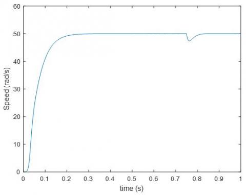
Figure 9. (a) Electromagnetic Torque for Cr=35N.m in 0.75s, (b) Speed response with adding a load torque resistant at time t=0.75s
In this part, the performance and effectiveness of the dual SVM three-phase multilevel inverter is achieved in order to drive a DSIM with IFOC. The DSIM parameters are investigated and exposed in the Appendix. Otherwise, Figure 9(a) presents an electromagnetic torque and Figure 9(b) shows the speed response after adding a load torque of Cr=35N.m at time t=0.75s with α=30. It is obvious from these figures that the machine speed signals tracks effectively the reference signal. Also, it can be seen from the obtained outcomes that when the load torque application is occurred at the instant t=0.75s, the speed decreasing is insignificantly appeared, but it is returned quickly once more devoid of error. This simulation results are noticeably proved the robustness of suggested scheme.
The torque magnitude is increased from 0 Nm to 35 Nm as depicted in Figure 9(a) and remained constant at 35 Nm as shown. Thus, the simulation results highlight the best control and attains the good performance of the system with the proposed scheme. It can be noted that the similar outcomes for α =30° and 0° as illustrated in the torque electromagnetic and the speed.
(a)
(b)
Figure 10. (a) currents stator of the DSIM (b) currents Zoom stator
Figure 10 is shown the stator current for α =30°. Primarily, in the beginning, the stator current is spotted to have emphatically rippled because of not using starting methods. It is noticeable that IFOC is achieved superior appropriate control to speed signal and demonstrated to be a great method for controlling the inconsistent speed drives.
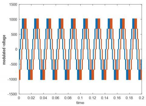
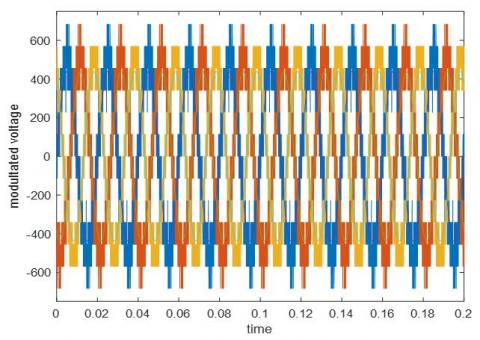
Figure 11(a) and (b) is exposed a five-level modulated voltage. It is clear to say that the obtained result establishes the effectiveness and robustness of the mentioned technique, and it displays the advantage of multilevel inverters that carry the output voltages with a low total harmonic distortion.
(a)
(b)
Figure 11. (a) Two modulated voltages, (b) Three modulated voltages
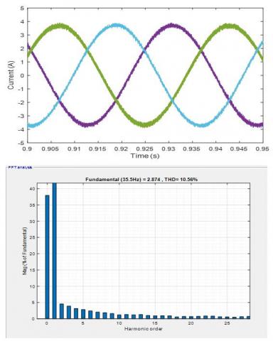
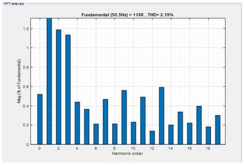
DSIM numerical outcomes for displacement amid stator winding (α=0°, 30° and 60°) is illustrated in Figure 12. Profoundly, Figure 12(a) presents the numerical outcomes of the five levels of the output currents for α=30°. Besides, The THD of this later is obtained as 10.19% by FFT analysis. In Figure 12(b), the achieved outcomes illustrate the five levels of the output currents for α=60°, where its THD is achieved as 10.39% by FFT analysis. Similarly, the mentioned results expose the five levels of the output currents for α=0° as showed in Figure 12(c). We can see that the THD value is obtained as 10.56%.
Figure 13(a), (b) and (c) shows the THD percentage according to the angle of α=30 with the changed frequency and. Whereas, Figure 13(d) displays the phase voltage for five-level. The mentioned results proves that when decreasing the levels number of frequency, the output voltage will be similar to the sinusoid shape as well as the THD decreases that produce least THD in the output voltage.
From the exposed outcomes, it is remarkable that the stator's currents are better and smooth under this strategy. Best THD is achieved with α=30° phase shift angle in level 5. Also, when the level number augments the output voltage signal becomes near to being more and more precise sinusoidal form. Consequently, the THD captured by FFT analysis in simulation results of the output voltage signal under α=30° is perfect and has little value which substantiates the effectiveness and applicability of the proposed strategy.
(a)
(b)
(c)
Figure 12. Percentage of the THD with different angle α =30,60,0 with Phase currents five -level for (a) α=30, for (b) α=60 and (c) α=0
(a)
(b)
(c)
(d)
Figure 13. (a), (b) and (c) Percentage of the THD to the angle α=30 with different frequency and (d) Phase voltage for five-level
In this paper, a robust strategy is firstly studied to control a DCMI by dual thee phase SVM and drive a DSIM. Secondly, the control of DSIM supplied by multilevel inverters associated to the IFOC technique is also applied. The numerical outcomes clearly reveal the superior effectiveness of the proposed scheme and prove the efficiency of the mentioned strategy in the high power synchronous motor drives. The output torque ripple and stator current harmonic losses are generally diminished. The principal benefit of phase shift employment α consists to appear that the dual three-phase SVM is general in any case of phase shift. An efficiency comparison is done based on phase currents and voltage THD analysis under various reference frequency and α angle. The obtained results are proved that the suggested scheme is appropriate for five level inverter and even any level inverter in case of using the common form. Also, this strategy is given better signal sinusoidal and little value of THD for the phase voltage and currents, especially when the level of inverter augmented. The advantage of this strategy scheme makes it a useful tool for further study of the power drive and multilevel inverter.
Machine parameters:
|
rated power |
Pn=5.5 kW |
|
rated current |
In=6 A |
|
rated voltage |
Vn=220 V |
|
number of poles |
P=6 |
|
rated speed |
Nn=1000 rpm |
|
rotor resistance |
Rr=3 Ω |
|
stator resistance |
Rs=2.03 Ω |
|
rotor inductance |
Lr=0.2147 H |
|
stator inductance |
Ls=0.2147 H |
|
mutual inductance |
M=0.2 H |
|
moment of inertia |
J=0.06 kg.m2 |
[1] Rodriguez, J., Franquelo, L.G., Kouro, S., Leon, J.I., Portillo, R.C., Prats, M.A.M., Perez, M.A. (2009). Multilevel converters: An enabling technology for high-power applications. Proceedings of the IEEE, 97(11): 1786-1817. https://doi.org/10.1109/JPROC.2009.2030235
[2] Alcharea, R., Nahidmobarakeh, B., Betin, F., Capolino, G.A. (2008). Direct torque control (DTC) for six-phase symmetrical induction machine under open phase fault. In MELECON 2008-The 14th IEEE Mediterranean Electrotechnical Conference, pp. 508-513. https://doi.org/10.1109/MELCON.2008.4618486
[3] Bojoi, R., Levi, E., Farina, F., Tenconi, A., Profumo, F. (2006). Dual three-phase induction motor drive with digital current control in the stationary reference frame. IEE Proceedings-Electric Power Applications, 153(1): 129-139. https://doi.org/10.1049/ip-epa:20050215
[4] Pan, D., Wu, H., Wang, F., Deng, K. (2008). Study on dual stator winding induction generator system based on fuzzy control. In 2008 IEEE Vehicle Power and Propulsion Conference, pp. 1-4. https://doi.org/10.1109/VPPC.2008.4677637
[5] Banala, T., Lakshman Rao, D. (2014). Simple and efficient SVPWM algorithm for diode clamped 3-level inverter fed DTC-IM drive. The International Journal of Engineering and Science, pp. 2319-1805.
[6] Blaschke, F. (1972). The principle of field orientation as applied to the new transvector closed loop control system for rotating-field machines. Siemens Review, 217-220.
[7] Casadei, D., Serra, G., Tani, K. (2000). Implementation of a direct control algorithm for induction motors based on discrete space vector modulation. IEEE Transactions on Power Electronics, 15(4): 769-777. https://doi.org/10.1109/63.849048
[8] Kim, S.H., Sul, S.K. (1995). Maximum torque control of an induction machine in the field weakening region. IEEE Transactions on Industry Applications, 31(4): 787-794. https://doi.org/10.1109/28.395288
[9] Li, F., Hua, W., Tong, M., Zhao, G., Cheng, M. (2015). Nine-phase flux-switching permanent magnet brushless machine for low-speed and high-torque applications. IEEE Transactions on Magnetics, 51(3): 1-4. https://doi.org/10.1109/TMAG.2014.2364716
[10] Karasani, R.R., Borghate, V.B., Meshram, P.M., Suryawanshi, H.M., Sabyasachi, S. (2016). A three-phase hybrid cascaded modular multilevel inverter for renewable energy environment. IEEE Transactions on Power Electronics, 32(2): 1070-1087. https://doi.org/10.1109/TPEL.2016.2542519
[11] Bentouhamia, L., Abdessemedb, R., Kessala, A., Merabeta, E. (2018). Control neuro-fuzzy of a dual star induction machine (DSIM) supplied by five-level inverter. Journal of Power Technologies, 98(1): 70-79. http://dx.doi.org/10.4236/jpt.2018.63001
[12] Grandi, G., Tani, A., Sanjeevikumar, P., Ostojic, D. (2010). Multi-phase multi-level AC motor drive based on four three-phase two-level inverters. In SPEEDAM 2010, pp. 1768-1775. https://doi.org/10.1109/SPEEDAM.2010.5545091
[13] Jones, M., Patkar, F., Levi, E. (2013). Carrier-based pulse-width modulation techniques for asymmetrical six-phase open-end winding drives. IET Electric Power Applications, 7(6): 441-452. https://doi.org/10.1049/iet-epa.2012.0372
[14] Kumar, A.S., Gowri, K., Kumar, M.V. (2018). New generalized SVPWM algorithm for multilevel inverters. Journal of Power Electronics, 18(4): 1027-1036. https://doi.org/10.6113/JPE.2018.18.4.1027
[15] Sadouni, R. (2020). Three level DTC-SVM for dual star induction motor fed by two cascade VSI with DPCVF-SVM Rectifier. Journal of Power Technologies, 100(2): 171-177.
[16] Hellali, L., Belmahdi, S., Loutfi, B., Hassen, R. (2018). Direct torque control of doubly star induction machine fed by voltage source inverter using type-2 fuzzy logic speed controller. Advanced in Modeling and Analysis C, 73(04): 202-207. https://doi.org/10.18280/ama_c.730410
[17] Bouziane, M., Abdelkader, M. (2019). Direct space vector modulation for matrix converter fed dual star induction machine and neuro-fuzzy speed controller. Bulletin of Electrical Engineering and Informatics, 8(3): 818-828. https://doi.org/10.11591/eei.v8i3.1560
[18] Lyas, B., Bouhali, O., Khadar, S., Mohammed, Y. (2019). A novel dual three-phase multilevel space vector modulation for six-phase multilevel inverters to drive induction machine. Modelling, Measurement and Control A, 92(2-4): 79-89. https://doi.org/10.18280/mmc_a.922-407
[19] Khemili, F.Z., Rizoug, N., Bouhali, O., Benjdaia, B., Lefouili, M. (2020). Balancing of state of charge batteries in a three phase diode clamped inverter controlled by a direct space vector of line to line voltages. 7th International Conference on Control, Decision and Information Technologies, CoDIT 2020. https://doi.org/10.1109/CoDIT49905.2020.9263832
[20] Bouhali, O., Francois, B., Berkouk, E.M., Saudemont, C. (2007). DC link capacitor voltage balancing in a three-phase diode clamped inverter controlled by a directspace vector of line-to-line voltages. IEEE Transactions on Power Electronics, 22(5): 1636-1648. https://doi.org/10.1109/TPEL.2007.904174
[21] Benalia, L., Chaghi, A., Abdessemed, R. (2011). Comparative study between a double fed induction machine and double star induction machine using direct torque control DTC. Acta Universitatis Apulensis, 28: 351-366.
[22] Boukhalfa, G., Belkacem, S., Chikhi, A., Benaggoune, S. (2019). Genetic algorithm and particle swarm optimization tuned fuzzy PID controller on direct torque control of dual star induction motor. Journal of Central South University, 26(7): 1886-1896. https://doi.org/10.1007/s11771-019-4142-3
[23] Salima, L., Tahar, B., Youcef, S. (2013). Direct torque control of dual star induction motor. International Journal of Renewable Energy Research, 3(1).
[24] Amimeur, H., Abdessemed, R., Aouzellag, D., Ghedamsi, K., Hamoudi, F., Chekkal, S. (2011). A sliding mode control for dual-stator induction motor drives fed by matrix converters. Journal of Electrical Engineering, 11(2): 8-8. https://doi.org/10.1109/TPEL.2007.904174