Salah Benzian* | Aissa Ameur | Aissa Rebai
© 2021 IIETA. This article is published by IIETA and is licensed under the CC BY 4.0 license (http://creativecommons.org/licenses/by/4.0/).
OPEN ACCESS
Diabetes is one of the most important diseases that researchers have focused on in scientific research since the time, because of the seriousness of this disease if it is not properly dealt with, especially with the emergence of some global epidemics such as Corona Virus (COVID 19), as the pancreas is the organ responsible for regulating sugar in the blood by secreting the insulin enzyme, insulin is widely used to control blood sugar. Therefore, it is important that the required insulin value is constant and controlled. The aim of this study is to control the blood glucose value that is achieved as a desired value and to maintain it as a constant value using a proportional, integral, and derivative control unit (FOPID) fractional order of the control parameters. In this research, the new control unit is applied to Bergman's mathematical model as a non-linear and simple model that simulates the mechanism of the interaction of glucose and insulin in the blood, and based on this, a closed control loop was designed to regulate the level of blood sugar to be an automatic control of blood glucose using the measured data from Special sensor. The contribution in this scientific paper is to define the (FOPID) parameters according to the closed loop responses of the system, and these parameters were adjusted using new meta-heuristic algorithms including the Invasive Weed Optimization (IWO), the PSO Particle Swarm optimization, the Genetic Algorithm (GA), The bat optimization algorithm (BA) and (ACO). As a result, the results of the five modern algorithms were compared based on several criteria to find out which one was better using MATLAB / SIMULINK simulation. It was found that the IWO algorithm performs better than PSO. The simulation results of the closed-loop system of this controller at the time of settling, overshoot and control inputs indicate very positive results compared to previous results. In addition, a new method has been proposed which is to design a pump in the form of a valve to control insulin pumping by controlling it with the fuzzy logic control unit, which in turn, we obtained better results, compared to the results of other previous studies.
Bergman minimal model, FOPID controller, fuzzy logic controller, fractional calculus, PSO, IWO, BA ACO and GA
Diabetes is considered one of the most health challenges in the world in the twenty-first century, As it has become a depleting human and material resources epidemic threatening both developing and developed countries, As the complications arising from it, such as cardiovascular diseases and diabetic neuropathy, all lead to a lower level of life [1, 2], And increase the economic burdens on the individual, the family, and then society as a whole [1-4], Especially with the emergence of some modern epidemics, such as COVID 19, as studies have shown that diabetics are the most common death from this epidemic.
According to the statistical forecasts of the International Diabetes Federation (IDF) and the World Health Organization (WHO), the number of diabetics in the world will reach in the year 2030 approximately 438 million [1, 2, 5].
Diabetes is a chronic metabolic disease that manifests itself with an increase in the level of sugar in the blood as a result of a relative or complete lack of insulin secreted by the pancreas into the blood [1, 2], or an imbalance in the strength of the effect of insulin on tissues that consume glucose, such as muscles, fatty tissue and the liver, and this frequent rise results in chronic complications in Different organs of the body.
There are two types of diabetes, type 2 and type 1, type 2 diabetes is characterized by the presence of insulin resistance by stored tissues that consume glucose sugar, such as the liver, muscles, and fatty tissues in the body [1, 2]. Patients with type 2 diabetes can usually regulate their condition through A balanced diet and exercise. As for the first type, it is characterized by the breakdown of the beta cells that secrete insulin in the pancreas through the autoantibodies that form in the patient’s blood, and thus are complete for the loss of insulin in the blood The body, but this injection is not sufficient[1, 3, 4, 6,], and based on these data and data, this topic was chosen by the researchers for its importance and opening the way for future studies about it, as a new device called the artificial pancreas was developed [7] in order to avoid type 1 diabetes and control the level of glucose. In the blood and keeping it in the normal level, and This importance increased with the emergence of the Coronavirus (COVID 19), because diabetics quickly became infected with this epidemic and died, so it became imperative to find quick solutions to diagnose and reduce this disease.
The artificial pancreas consists of three main parts: i) a automatic pump, ii) an in vivo glucose sensor; and iii) a mathematical algorithm to adjust the pump given a sensor measurement [3, 4, 6]. By controlling the closed loop, this type of closed-loop system technology provides continuous control of blood sugar without the use of hands and facilitates the life of diabetics [7, 8], Also in a closed loop control system the patient needs to use a glucose sensor that can measure the blood glucose level. Immediately afterwards, this information is passed to a control device that calculates the rate of insulin delivery needed to keep the blood glucose level in a constant range via a mechanical pump that can deliver the required amount of insulin [7, 8]. In general, the closed loop method is more reliable in maintaining the level of glucose in the blood, as it closely mimics a healthy pancreas.
In recent years, many mathematical studies and models have been conducted on this topic, and among the mathematical models is the non-linear model of Bergman [8, 9], which is the subject of our study, He is considered the first person to provide a basic and proven physiologically mathematical model for controlling blood glucose in the human body [3, 4, 6].
There are many previous studies that have dealt with this topic using the Bergman model, controlling it and dealing with it from different angles, including the use of the classical controller (PID) provided by Ramprasad, Y, Rangaiah, G in 2004 and others for example [10-16].
Also suggested Ibbini [14] and his colleagues in 2004 a control closed-loop with the optimal way to develop the Bergman model to improve the status of glucose in the blood in patients with diabetes.
In 2019, H. Heydarinejad and his colleagues proposed a new combination of fractional order (FO) nonlinear control and Fuzzy type-2 fractional Backstepping blood glucose control based on sliding mode observer is proposed [15, 16].
And Some of control algorithm proposed traditional techniques such as pole placement [17, 18] Optimal control using algorithms [12, 14, 19-21], or some robust approaches such as H∞ control [8, 9, 20-24], or predictive control and realization of model [3, 25] but it did not rise to the required level.
And By setting Simulation of a model based on fuzzy control system for Glycemic Control in Diabetes introduced by Boldisor, C., &Coman, S in 2015 [22].
Sohaib Mehmood [2] in the year 2020 also used a good comparison of some control techniques, but this paper lacked graphs in order to know the importance of these techniques.
On the other hand, Parsa [9] proposed, in the year 2020, a modern algorithm (Grasshopper Optimization Algorithm (GHO)) to improve the parameters of the classic control unit (PID Controller) to control the level of glucose and compared it with some algorithms. However, this work did not explain the importance of these techniques with graphs and did not address the fractional control unit (FO-PID Controller).
Since the application of fractional calculus is important in control engineering through modeling and control design due to its ability to improve the performance of closed-loop systems and increase robustness, the fractional order controllers are considered a design substitute to classical controllers and one of the main advantages is better system characterization [26, 27]. and increased flexibility. $P I^{\lambda} D^{\mu}$ fractional order is important for improving closed-loop performance, and being able to meet more performance specifications as well as increased durability compared to the classical PID controller [26, 27]. That is why our contribution to this research was on the application of a FOPID controller for good blood glucose control, closed loop control, and good response determination respectively. By finding a better solution by applying several new meta-heuristic algorithms including the Particle Swarm Optimization (PSO) [28, 29], The bat optimization algorithm (BA), Invasive Weed Optimization (IWO) [30, 31], Ant Colony Optimization (ACO) [32]. and technology Genetic algorithm (GA) [33]. As a result, we also focused on comparing the efficiency of the results of the five new techniques based on several criteria, including stability time, overshoot and steady state error, in order to find out good algorithms using MATLAB / SIMULINK simulation.
In addition, a new method has been proposed, represented in designing a pump in the form of a valve to control insulin infusion by controlling it with a fuzzy logic controller to regulate the level of glucose in the blood, and the results we obtained showed that There are better results for good blood glucose control compared to results from other previous studies.
In the beginning, we gave a comprehensive overview of the basic concept of fractional calculus in the first section. The second section discusses the Type 1 diabetes model, the Fractional -Order Controller $P I^{\lambda} D^{\mu}$ is described in the third section, Parameter Tuning using Optimization Technique detailed in the fourth section, Applications of algorithms searches, and analyzing the results and discussing them in the fifth and sixth sections, Fuzzy logic controller for blood glucose concentration and discussion of its results detailed in the seventh section.
Fractional order calculations participate a very important function in various scientific fields, particularly in the last decade, the application of fractional order control in control engineering has been raised as an important topic in the field of international research [34-38]. Recently, scientists have shown that fractional order equations are capable to model various phenomena more suitably than the correct order [37, 38]. The most commonly used and important definitions for fractional order derivatives and integrals are Granwald-Letnikov, Riemann, Leville 8, and Caputo [35-38].
Fractional calculus is a generalization of the derivative of a function and its integral over an incorrect order [29, 37, 39]. In geometry, the fractional order α is often less than 1, 0<α<1.
2.1 Definition 1
The Riemann–Liouville (RL) fractional derivative of order ${\alpha} \in(0,1)$ of m(t) is given by [35], or [38].
$\mathrm{RL}_{\mathrm{t}_{0}} \mathrm{D}_{\mathrm{t}}^{\alpha} \mathrm{f}(\mathrm{t})=\frac{1}{\Gamma(1-\alpha)} \frac{\mathrm{d}}{\mathrm{d} \mathrm{t}} \int_{\mathrm{t}_{0}}^{\mathrm{t}}(\mathrm{t}-\mathrm{s})^{-\alpha} \mathrm{F}(\mathrm{s}) \mathrm{ds}, \mathrm{t} \geq \mathrm{t}_{0}$ (1)
where, the Euler-Gamma function is defined as follows:
$\Gamma(\alpha)=\int_{0}^{\infty} e^{-\alpha} u^{\alpha-1} d u ; \alpha \in R$ (2)
2.2 Definition 2
(Caputo fractional derivative [1]). The Caputo fractional derivative of order a 2 R on the half axis R is defined as follows [35-38]:
${ }_{a}^{c} D_{t}^{\alpha} f(t)$$=\left\{\begin{array}{c}\frac{1}{\Gamma(m-\alpha)} \int_{a}^{t} \frac{f^{(m)}(\tau)}{(t-\tau)^{\alpha+1-m}} d \tau m-1<\alpha<m \\ \frac{d^{m}}{d t^{m}} f(t) \alpha=m\end{array}\right.$ (3)
with $\mathrm{m}=\min \{\mathrm{k} \in \mathrm{N} / \mathrm{k}>\alpha\}, \alpha>0$;
2.3 Lemma 1
The Laplace transform of the Caputo fractional derivative of order m; $1<\alpha<m$ is [35-38]:
$L\left\{{ }_{c} D_{q}^{\alpha} f(t)\right\}=s^{\alpha} L\{f(t)\}-\sum_{k=0}^{m-1} s^{\alpha-k-1} f^{(k)}(q)$ (4)
Within the human body, glucose is regulated and its level controlled at a safe value in the body by the pancreas. When the level of sugar in the body rises, insulin is pumped through the pancreas into the liver and then pumped into the blood through the liver, and so on until the level of glucose in the blood is maintained at the desired level [1, 2, 34].
In this section, a mathematical dynamic model is described. It is based on Bergman's Minimal Model, which was used to describe the relationship between glucose and insulin by Richard Bergmann in 1980 [4, 6]. This model was first developed by the Ackermann Group. What distinguishes this system also is that it is used to design the desired control unit and simulation, and it is one of the famous simple mathematical models that are non-linear and has sufficient credibility in the main laboratories in the world [1, 2, 34], and thus it explains the dynamic response to blood glucose concentration in type 1 diabetics as this model consists of three equations Differential shown as follows [1, 2, 40-42]:
$\dot{G(t)}=p_{1}\left[G(t)-G_{b}\right]-X(t) G(t)+D(t)$ (5)
$\dot{X(t)}=-\mathrm{p}_{2} \mathrm{X}(\mathrm{t})+\mathrm{p}_{3}\left[\mathrm{I}(\mathrm{t})-\mathrm{I}_{\mathrm{b}}\right]$ (6)
$\dot{\mathrm{I}(\mathrm{t})}=-\mathrm{n}\left[\mathrm{I}(\mathrm{t})-\mathrm{I}_{\mathrm{b}}\right]+\gamma[\mathrm{G}(\mathrm{t})-\mathrm{h}]^{+} \mathrm{t}+\mathrm{u}(\mathrm{t})$ (7)
where, that the initial conditions of the above three differential equations are as the following:
$\mathrm{G}(0)=\mathrm{G}_{0}, \mathrm{x}(0)=0, \mathrm{I}(0)=\mathrm{I}_{0}$
And The parameters of differential equations are defined [4, 6, 29] in Table 1.
D(t) Meal glucose disorder (mg/dL/min), after eating. Due to the absence of a pancreas to regulate natural insulin in patients with diabetes, this glucose uptake is considered to be a disturbance of the system dynamics presented in Eq. (1). The function $\mathrm{D}(\mathrm{t})$ in diabetic patients is presented at [22] as:
$D(t)=A \exp (-B t) ; B>0$ (8)
where, t is the time in (min) and D(t) is in (mg/dl/min).
In our work we take D(t) as:
$D(t)=0.5 \exp (-0.05 t)$ (9)
U(t)-rate of treated insulin infusion (mU/min) to control insulin which is considered the organization of natural insulin to the body system.
$\operatorname{tmax}=$80 min is the time at which the peak value of glucose absorption.
Table 1. Meaning parameters of the model
|
Parameter |
Description |
|
t |
Time[min] |
|
G(t) |
Blood glucose Concentration[mg/dL] |
|
$\mathbf{G}_{\mathbf{b}}, \mathbf{I}_{\mathbf{b}}$ |
The basal pre injection level of glucose [mg/dL] and insulin[mU/L] in blood, respectively (baseline) [mg/dL] |
|
I(t) |
Active insulin concentration[mU/L] |
|
X(t) |
The effect of Active insulin. [1/min] |
|
I(t) |
Blood insulin concentration |
|
n |
The Time constant for insulin in plasma (1/min) |
|
h |
The threshold value of glucose above which the pancreatic β-cells release insulin (mg/dl) |
|
$\gamma$ |
The rate of the pancreatic β-cells’ release of insulin after the glucose injection with glucose concentration |
|
P1 |
Insulin-independent rate constant of glucose uptake in muscles and liver in (1/min) |
|
P2 |
Rate for decrease in tissue glucose up take ability (1/min) |
|
P3 |
Insulin dependent increase in glucose uptake capacity in tissues per unit of insulin concentration above basal level in $\left(\frac{\mu U}{m l}\right)^{-1} m^{-1}$ |
This system is a nonlinear system, after analyzing it and converting it to Laplace Transform, we get the following Transfer function:
$\begin{aligned} \frac{G(s)}{U(s)}=& \frac{-p_{3} G_{b}}{s^{3}+s^{2}\left(n+p_{1}+p_{2}\right)} \\ &+s\left(n p_{1}+n p_{2}+p_{1} p_{2}\right)+n p_{1} p_{2} \end{aligned}$ (10)
As the parameters n, $\mathrm{p}_{1}, \mathrm{p}_{2}, \mathrm{p}_{3}, \mathrm{G}_{\mathrm{b}}$, differ from one person to another according to the health and disease of the human being and are listed in Table 2 [6].
Table 2. Model parameter values
|
Parameter |
Normal |
Patient 1 |
Patient 2 |
Patient 3 |
|
P1 |
0.031 |
0 |
0 |
0 |
|
P2 |
0.012 |
0.011 |
0.007 |
0.014 |
|
P3 |
$4.92^{-6}$ |
5.3-6 |
2.16-6 |
9.94-6 |
|
$\gamma$ |
0.0039 |
0.0042 |
0.0038 |
0.0046 |
|
n |
0.265 |
0.26 |
0.246 |
0.281 |
|
h |
79.035 |
80.2 |
77.578 |
82.937 |
|
$\mathbf{G}_{\mathbf{b}}$ |
70 |
70 |
70 |
70 |
|
$\mathbf{I}_{\mathbf{b}}$ |
7 |
7 |
7 |
7 |
|
$\mathbf{G}_{\mathbf{0}}$ |
291.2 |
220 |
200 |
180 |
|
$\mathbf{I}_{\mathbf{0}}$ |
364.8 |
50 |
55 |
60 |
PID control is the method most widely used technique today in industrial process control which is defined as the relative integral derivative which can be defined mathematically using the differential equation [10, 21]:
$u(t)=k_{p} e(t)+k_{i} \int_{0}^{t} e(\tau) d \tau+k_{d} \frac{d e(t)}{d t}$ (11)
When performing the Laplace transform of Eq. (11), which is the equation of the PID controller, its transfer function is well known in the form [10, 21]:
$U(S)=k_{p}+\frac{k_{i}}{S}+k_{d} S$ (12)
where, Kp: is the gain of proportionality, Ki: is the gain of Integral, Kd: is the gain of Derivative.
e: is the Error, t: is the instantaneous time and τ: is the variable of integration that takes on the values from time 0 to the present t.
And E(S): is the error and U(S): is the command.
4.1 FOPID ( $\mathbf{P I}^{\lambda} \mathbf{D}^{\boldsymbol{\mu}}$ ) controller
After the discovery of fractional calculus, it has been applied in many fields, including the field of control theory [38, 34]. Thus, FOPID controllers have become of great interest in recent years because of their good advantages, including flexibility in design and good performance compared to classic PID controllers, because they have five parameters for tuning. Other than the control parameters Kp, Ki, and Kd of a regular PID controller there are λ and μ, the fractional powers of the integral and derivative parts respectively. It can be defined mathematically using the following differential equation [31, 32]:
$u(t)=k_{p} e(t)+k_{i} D^{-\lambda} e(t)+k_{d} D^{u} e(t)$ (13)
By applying the Laplace transform to Eq. (13). with the initial conditions zero, the transfer function of this Controller could be expressed by:
$U(S)=k_{p}+\frac{k_{i}}{S^{\lambda}}+k_{d} S^{u}$ (14)
All these types of classical PID controllers are special cases of the $P I^{\lambda} D^{\mu}$ controller defined and given in Eq. (14). Thus the $P I^{\lambda} D^{\mu}$ Controller Generalize the classical PID controller.
In this section we introduce the Particle Swarm Optimization (PSO), The bat optimization algorithm (BA), Invasive Weed Optimization (IWO), Ant Colony Optimization (ACO) and technology Genetic algorithm (GA) for tuning FOPID controller parameters. The major objective of this function is to reduce the steady state error so that the closed-loop system is internally stable. Hence, we dealt with making a comparison between all the methods in the simulation results using MATLAB.
5.1 Particle Swarm Optimization (PSO)
The Particle Swarm Optimization (PSO) algorithm is an optimal technology developed during the 1995's by James Kennedy and Eberhart, [9, 28, 29] and others and is a heuristic approach inspired by observing the social behavior of bird flow and fish education. Initial ideas about particle swarm are based on producing computational intelligence that mimics social improvement. This simulation was formulated in flocks of birds searching for corn by Heppner and Grenander's [9, 28, 29].
Particle Swarm Optimization (PSO) is a powerful optimization technique based on swarm intelligence as an algorithm inspired by nature. Its basic concept is to use a number of particles containing a swarm that moves and searches for the best solution in the problem space. Each particle in the search space modifies its ability to fly and its experience with other particles [28]. The goal of PSO is to optimize continuous nonlinear functions to find the best solution in the problem space. Several studies have proven to be highly effective in dissolving solutions in various engineering and research applications [9, 28, 29].
The concept of improving particle swarm at every time step includes changing the velocity of each particle towards the best global and local locations [28, 29].
The speed of each particle is adjusted according to its own flying experience and the flight experience of other particles. The i-th particle is represented as:
The best indicator particle among all the particles in the group is gbest. The velocity for particle i is represented as:
$\mathrm{v}_{\mathrm{i}}=\left(\mathrm{v}_{\mathrm{i}, 1}, \mathrm{v}_{\mathrm{i}, 2}, \ldots \ldots \ldots . \mathrm{v}_{\mathrm{i}, \mathrm{d}}\right)$ (15)
The adjusted velocity and position of each particle can be calculated using the current velocity and distance from $\mathrm{x}_{\mathrm{i}, \mathrm{d}}^{\mathrm{b}}$ and to gbest as shown in the following Eq. (16), (17).
$v_{i}^{k+1}=w v_{i}^{k}+c_{1} \operatorname{rand}\left(x_{i}^{b}-x_{i}^{k}\right)$$+c_{2} \operatorname{rand} \times\left(x_{i}^{g}-x_{i}\right)$ (16)
$x_{i}^{k+1}=x_{i}^{k}+v_{i}^{k+1}$ (17)
$v_{i}^{k}$: velocity of agent i at iteration k.
W: weighting function.
$\mathrm{C}_{\mathrm{J}}$: weighting factor.
rand: uniformly distributed random number between 0 and 1.
pbesti: pbest of agent i. gbest: gbest of the group.
5.2 The BAT optimization algorithm (BA)
The bat optimization algorithm (BA) is a powerful optimization technique and its capabilities are based on the intelligence of bats. It was proposed by the researcher Yang 19, as it is an algorithm inspired by nature [40, 41]. Its basic concept is to use a number of particles that contain the bats ’ability to move and search, such as finding their prey and distinguishing Between different types of insects even in complete darkness. Thus, bats, especially small bats, can recognize the positions of objects by spreading high and short sound signals and by colliding and reflecting these propagation signals [40, 41]. BA differs from other swarm intelligence improvement techniques with the loudness and pulse emission rate values in the refresh value of the BA parameter equations.
1-All bats use echolocation to sense distance and magically know the difference between food / prey and back barriers;
2-Bats fly randomly at $\mathrm{Vi}$ in position $\mathrm{X}_{\mathrm{i}}$ with $\mathrm{f}_{\mathrm{min}}$ frequency, variable wavelength and loudness $\mathrm{A}_{0}$ to search for prey. They can adjust the wavelength (or frequency) automatically emitted pulses and adjust the rate of emission of pulses r [0, 1], depending on the near goal; [40, 41].
3-The velocity of each population (N) is calculated using,
$\mathrm{v}_{\mathrm{i}}^{\mathrm{t}}=\mathrm{v}_{\mathrm{i}}^{\mathrm{t}-1}+\left(\mathrm{x}_{\mathrm{i}}^{\mathrm{t}}-\mathrm{x}_{*}\right) \mathrm{f}_{\mathrm{i}}$ (18)
$\mathrm{x}_{\mathrm{i}}^{\mathrm{t}}=\mathrm{x}_{\mathrm{i}}^{\mathrm{t}-1}+\mathrm{v}_{\mathrm{i}}^{\mathrm{t}}$ (19)
4-The frequency of the signals sent is calculated by each of the bats [30, 31]:
$\mathrm{f}_{\mathrm{i}}=\mathrm{f}_{\min }+\left(\mathrm{f}_{\max }-\mathrm{f}_{\min }\right) \beta$ (20)
where, β in the range of [0, 1] is a random vector drawn from a uniform distribution and $\mathrm{X}_{*}$ is the current global best location. Every bat is randomly assigned a frequency which is drawn uniformly from ($\mathrm{f}_{\mathrm{max}}, \mathrm{f}_{\mathrm{min}}$) A random walk around the current best solutions is known as the local search. Where a novel solution for every bat can be generated locally by [40, 41].
$x_{\text {new }}=x_{\text {old }}+\varepsilon A^{t}$ (21)
where, $\varepsilon[-1,1]$ is a scaling factor which is a random number, while $A^{t}$ is the average loudness of all bats at time step. the loudness and the rate of pulse emission will be updated accordingly by using Eq. (21).
$A_{i}^{t+1}=\alpha A_{i}^{t}, r_{i}^{t+1}=r_{i}^{0}\left[1-e^{(-\gamma t)}\right]$
Bat algorithm
Objective function $f(x), x=(x 1, \ldots, x d) T$
Initialize the bat population $x i$ (i=1, 2,........, n) and vi
Define pulse frequency fi at $x i$
Initialize pulse rates ri and the loudness Ai
while (t <Max number of iterations)
Generate new solutions by adjusting frequency,
and updating velocities and locations/ best solutions
if ( rand $>r i$)
Select a solution among the best solutions
Generate a local solution around the selected best solution
end if
Generate a new solution by flying randomly
if ($($ rand $<A i \& f(x i)<f(x *)$)
Accept the new solutions
Increase ri and reduce Ai
end if
Rank the bats and find the current best x∗
end while
Postprocess results and visualization
5.3 Invasive Weed Optimization (IWO)
IWO is a new evolutionary computational algorithm that relies on the natural behavior of weeds in searching for a suitable place for growth and reproduction by simulating the reproductive and growth behaviors of weeds in nature as the IWO algorithm is a random numerical search algorithm that IWO searches for the optimal solution to the problem in the solution space. In general, its most important steps in the calculation are based on four steps: initialization, cloning, spatial dispersion, and selection, which are as follows [30, 31].
5.3.1 Initialization
The primary group with Nwo-weed individuals is randomly generated in the D dimensional search space where each herb composed of variants represents a possible solution. After that, all WJ grass in the community reproduces seeds, and the seeds grow into multiple weeds through spatial dispersal. The amount (Nsj) of seeds produced by WJ is calculated using the following equation [30, 31]:
$\mathrm{N}_{\mathrm{S}_{\mathrm{j}}}=\frac{\mathrm{F}_{\mathrm{i}} \mathrm{t}_{\mathrm{j}}-\mathrm{F}_{\mathrm{i}} \mathrm{t}_{\mathrm{min}}}{\mathrm{F}_{\mathrm{i}} \mathrm{t}_{\mathrm{max}}-\mathrm{F}_{\mathrm{i}} \mathrm{t}_{\min }} \cdot\left(\mathrm{N}_{\mathrm{S}_{\max }}-\mathrm{N}_{\mathrm{S}_{\min }}\right)$$+\mathrm{N}_{\mathrm{S}_{\mathrm{min}}} \ldots .$ (22)
where, $\mathrm{F}_{\mathrm{i}} \mathrm{t}_{\mathrm{j}}$ is the fitness value of Wj; Fitmin and Fitmax are the minimum and maximum fitness values in the weed population, respectively; Nsmin and Nsmax are the minimum and maximum of the number of seeds, respectively.
5.3.2 Reproduction
The cloning process lies in the fact that the parent weeds with high fitness values produce more seeds, as the well-fit individual has a large capacity for production, as Nwmax grasses with high fitness values are selected from all weeds as the mother weed for the next iteration. By repeating Itermax times, weeds with the highest fitness value are the perfect solution to the problem. The formula is as follows [30, 31]:
$\operatorname{num}(i)=\frac{f_{i}-f_{w}}{f_{g}-f_{w}} *\left(s_{\max }-s_{\min }\right)+s_{\min }$ (23)
where, num(i) is the number of seeds for individual i (i=1, 2, …, N), fi is the fitness of the current weed, and fg and fw represent the members of the current population with the highest and lowest fitness, respectively
5.3.3 Spatial dispersal
At this stage, the seeds produced by the group are produced and spread according to the normal distribution with an average value of 0 and a standard deviation of its value. Thus, the fall of a grain in the range decreases non-linearly at each step, which leads to more suitable plants and the elimination of inappropriate plants the deviation update formula is as follows:
$\sigma_{\mathrm{t}}=\left[\frac{\mathrm{it}_{\mathrm{max}}-\mathrm{it}}{\mathrm{it}_{\mathrm{max}}}\right]^{\mathrm{n}} *\left(\sigma_{\mathrm{i}}-\sigma_{\mathrm{f}}\right)+\sigma_{\mathrm{f}}$ (24)
seed $_{\mathrm{i}, \mathrm{t}}=$mod(parent'sposition $\mathrm{w}_{\mathrm{i}}$$\left.+\operatorname{round}\left(\sigma_{\mathrm{t}} * \operatorname{randn}(0,1)\right), 4\right)$ (25)
where, $\sigma_{\mathrm{t}} \mathrm{rt}$ is the current standard deviation, it is the current iteration number, itmax is the maximum number of iterations, $\sigma_{i}$ and $\sigma_{f}$ are the initial and final standard deviation values, respectively, and n is a nonlinear factor. Mod function is a function of the remainder. Thus, Mod(number; divisor) returns the remainder after the number is divided by a divisor[30, 31].
5.3.4 Competitive exclusion
After several iterations if the number of weeds exceeds the maximum as the number of weeds and seeds reaches the maximum Nmax the weeds of worse fitness are removed from the colony and those of better fit will survive.
5.4 Ant Colony Optimization (ACO)
Ant colony optimization algorithms (ACO) are algorithms inspired by ant behavior. This algorithm was proposed in the 1990s by Marco Dorigo et al, to search for optimal pathways and methods based on a graph to solve many optimization problems. Ants are searching for a path between the colony of ants and their source of food to find the shortest path, individually or collectively, as follows:
The idea of an algorithm [32].
$\tau(\mathrm{k})_{\mathrm{ij}}=\tau(\mathrm{k}-1)_{\mathrm{ij}}+\frac{0.01 \theta}{\mathrm{J}}$ (26)
where, $\tau(\mathrm{k})_{\mathrm{ij}}$ is pheromone value between nest i and j at kth iteration, θ is the general pheromone updating coefficient and J is the cost function for the tour travelled by the ant.
Pheromones of the path belonging to the best tour and worst tour of the ant colony are updated as follows [32]:
$\tau(\mathrm{k})_{\mathrm{ij}}^{\text {worst }}=\tau(\mathrm{k})_{\mathrm{ij}}^{\text {worst }}-\frac{0.3 \theta}{\mathrm{J}_{\text {worst }}}$ (27)
$\tau(\mathrm{k})_{\mathrm{ij}}^{\mathrm{best}}=\tau(\mathrm{k})_{\mathrm{ij}}^{\mathrm{best}}-\frac{\theta}{\mathrm{J}_{\text {best }}}$ (28)
where, $\tau^{\text {best }}$ and $\tau^{\text {Worst }}$ are the pheromones of the paths followed by the ant in the tour with the lowest cost value $J_{\text {best }}$ and with the highest cost value $J_{\text {worst }}$ in one iteration respectively. After pheromone evaporation the ant algorithm forget its history and directed to search towards new direction without being trapped in some local minima as [32].
$\tau(\mathrm{k})_{\mathrm{ij}}=\tau(\mathrm{k})_{\mathrm{ij}}^{\lambda}+\left[\tau(\mathrm{k})_{\mathrm{ij}}^{\mathrm{best}}+\tau(\mathrm{k})_{\mathrm{ij}}^{\mathrm{worst}}\right]$ (29)
where, λ is a evaporation.
5.5 Genetic Algorithm (GA)
Genetic algorithm (GA) is a metaheuristic algorithm that relies on a random search technique using parametric coding; it is the process of searching for the most suitable chromosomes that constructed populations in the potential solution space. It aims to search for the best solutions and expand the search area. Thus, GA has become a powerful improvement tool for solving problems related to various fields of technical and social sciences [33] and has more detail in the following scientific research [33].
All the technical methods we mentioned were implemented as a M –file interconnected with the simulation model where the parameters of the FOPID controller are calculated and the optimization was performed to search for the five parameters of the fractional Order. The FOPID controller (Kp, Ki, Kd, λ and μ) was obtained directly according to the minimum of the value of the Fitness function, (ISE) and ((IAE)) shown in Table 3.
Also, for the model, the parameters of patient1 were chosen in the Bergman model, shown in Table 2.
such that so that:
(IAE) is the Total absolute value of error:
$\mathrm{IAE}=\int_{0}^{\infty}|\mathrm{e}(\mathrm{t})| \mathrm{dt}$ (30)
(ISE) is the Total square of error:
$I S E=\int_{0}^{\infty}(e(t))^{2} d t$ (31)
In this part, the criteria for these algorithms that have been used in the search results are given as follows:
6.1 Particle swarm optimization algorithm
FO-PID Controller parameters were found using PSO. Where is the closed-loop blood glucose level response found using parameters previously constructed in MATLAB? By using PSO standards. As follows:
m=5; number of variables
n=20; population size
$w_{\max }=0.9$ ; inertia weight
$W_{\min }=0.4$; inertia weight
c1=2; acceleration factor
c2=2; acceleration factor
maxite=100; set maximum number of iterations
maxrun=1; set maximum number of runs need to be
6.2 The Bat Optimization Algorithm (BA)
FOPID controller parameters were found using BAT. Where is the closed-loop blood glucose level response found using parameters previously constructed in MATLAB? By using BAT standards. As follows:
n=30; Population size, typically 10 to 40
N_gen=100; Number of generations
A=0.5; Loudness (constant or decreasing)
r=0.5;Pulse rate (constant or decreasing)
Qmin=1; Frequency minimum
Qmax=1; Frequency maximum
6.3 Invasive Weed Optimization (IWO)
FOPID controller parameters were found using IWO. Where is the closed-loop blood glucose level response found using parameters previously constructed in MATLAB. By using IWO standards. As follows:
nVar=5; Number of Decision Variables
MaxIt=200; Maximum Number of Iterations
nPop0=10; Initial Population Size
nPop=25; Maximum Population Size
Smin=0; Minimum Number of Seeds
Smax=5; Maximum Number of Seeds
Exponent=2;Variance Reduction Exponent
sigma_initial=0.5; Initial Value of Standard Deviation
sigma_final=0.001; Final Value of Standard Deviation
6.4 Ant Colony Optimization (ACO)
FOPID controller parameters were found using ACO Where is the closed-loop blood glucose level response found using parameters previously constructed in MATLAB. By using ACO standards. As follows:
n_iter=100; number of iterations
NA=30; Number of Ants
alpha=0.8;alpha
beta=0.2; beta
roh=0.7; Evaporation rate
n_param=5; number of parameters
n_node=1000;number of nodes for each parameter
6.5 The Genetic Algorithm (GA)
FOPID controller parameters were found using GA. Where the closed-loop blood glucose level response is found using parameters previously constructed in MATLAB. By using GA standards. As follows:
Number of Population 100
Crossover Operator 0.5
Mutation Operator 0.03
Length of Chromosome 67 Bit
Sensitivity of Variables 5
Number of Iteration 100
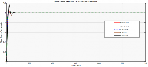
In this paper, we present five different algorithms that were used to find the five parameters of the FOPID controller. This is to control the level of glucose in the blood at a desired level by the form of responses shown in Figures 4, 5.
The numerical values of the parameters of the Bergmann Minimal Model vary according to each patient with type 1 diabetes and according to the disorders that occur within the body, as for the numerical values of the parameters of the Bergman model that we used in the simulations are shown in Table 2.
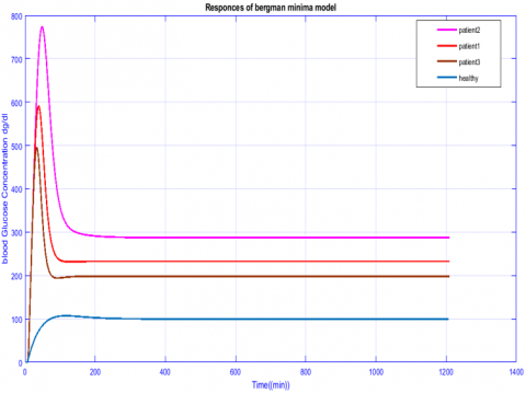
At the beginning of our study, we performed an open-loop simulation of the Bergman model according to the healthy person and each patient person, using the parameters listed in Table 2. For meal disturbances, we chose the equation as follows: $D(t)=0.05 e^{-0.05(t)}$ At time t=80 min, the results obtained are shown in Figure 2.
According to the results obtained from the data shown in Figure 2 the modeling validity of Bergman model showed that it is completely consistent with the available data, as we noticed that in the case of patient, the value of glucose rose to the highest level 750 [mg/dL] and decreased to the value 200 [mg/dL] which are values that indicate the presence of an abnormality in the level of glucose, As for the values relating to the healthy person, glucose has stabilized at the value of 100 [mg / dl].
After the nonlinear system Bergman is solved, FO-PID controllers are used to control the level of blood glucose. The main goal of FO-PID controller is to reduce the error between the actual process variable to the system reference. The common FO-PID control unit equation used in this study is given above as in Eq. (14). The methods used to tuning parameters of FO-PID controller are 5 new met heuristic Algorithms such as Particle Swarm Optimization (PS0), Invasive Weed Optimization (IWO), Bat Algorithm (BA), Ant Colony Optimization (ACO), and Genetic Algorithm (GA).
The results obtained are shown in Table 3, where Table 3 shows the performance of the algorithms according to the values of Overshoot, rise time, steady-state error according to the performance of the fitness function of each (IAE, ITAE, and ISE), System responses to controlling blood glucose levels are shown in Figure 4 and 5.
Figures 4 and 5 clearly show that each FO-PID based design has outperformed the PID controller, compared to the results of previous studies in [6, 7, 19].
Table 3 also shows the importance of the five algorithms in finding FO-PID parameters, as the results showed that these algorithms have an effective role in finding FO-PID parameters with good performance and stability in the reference value, and also showed that the differences in their effectiveness and performance are not very large, however it was noted that there are slight differences Among these algorithms in several criteria, for example the steady-state error, and the Overshoot value for all fitness functions, the IWO algorithm and the PSO algorithm showed performance over the rest of the algorithms.
On the other hand, there was a good decrease in the overshoot value for PSO, IWO and BA. The overshoot value has reached at IWO algorithm 1.4785% and PSO 1.6157%. This is for the IAE fitness function as shown in Figure 5. As for the ISE fitness function as shown in Figure 4, The overshoot value has reached 1.4041% at IWO and 1.5082%. These are very good results.
Moreover, we noticed that the IWO and PSO Algorithms also have a positive role in reducing the error, but with reference to the value of the settling time and the value of the rise time, we note that there is an advantage of the IWO Algorithm over the PSO Algorithm.
However, there are no significant differences between them, for example the difference in terms of fitness function performance relative to IAE and the maximum value of best IWO algorithm and worst GA algorithm is only 0.017,
We can say that the FO-PID-based controller is better than the PID controller, and this is by comparing us with the results of previous studies in Refs. [19, 33], and that the FO-PID controller based on the five aforementioned algorithms plays an effective role and gives a good response better than the FO-PID Controller, and this is compared to previous studies and results in Refs. [20, 34].
And in the end, compared to the five algorithms we can say: IWO and PSO algorithms have better and faster performance compared to other algorithms, thus, IWO and PSO can easily handle non-linear and non-differential objective functions.
And unlike GA and other algorithms, IWO and PSO are not so sensitive to starting point that they start anywhere in the search space, and ensure convergence of the algorithm with the optimal solution.
As for IWO and PSO, we noticed that there is better performance for IWO over PSO algorithm, albeit with a little bit.
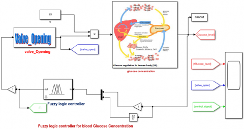
The main goal in this part is to design a pump to regulate the flow of insulin inside the body according to the level of glucose present in the blood, by controlling it with the fuzzy logic controller.
The controlled system is mathematically represented by the Bergman system.
The element that controls the pump is the valve, which is called ((Final control element FV)), which controls the change of glucose by pumping or determining the level of insulin entry into the body.
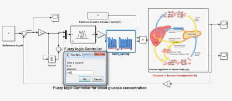
The fuzzy logic controller controls the valve opening as shown in Figure 1a.
In the beginning we dealt with the system on the basis of having a single Input and single output
For the input represented in glucose, expressed in mg/dl, we represent it by three membership functions (low, high and normal) and the output is represented by the valve opening we represent it by three membership functions (Close fast, Open fast and No change).
8.1 Fuzzy rules
Rule 1:→If Glucose level is normal, then valve is no change.
Rule 2:→If Glucose level is low, then valve is close fast.
Rule 3:→If Glucose level is high, then valve is open fast.
After implementing the system on Matlab Smulink, we obtained the Responses shown in Figure 6.
We notice that there is stability in the value 100 mg/dl and we also noticed that there is a too large overshoot and slow responses and the stability was a somewhat late.
To improve the performance and stability of the system at any desired glucose value or level, faster and less overshoot, we applied the closed loop system as shown in Figure 1b and tried to enter two inputs, namely (error level for blood glucose and error rate for blood glucose)), To this we also added the membership functions and Rules.
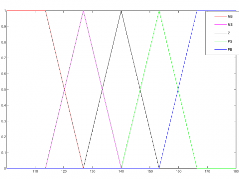
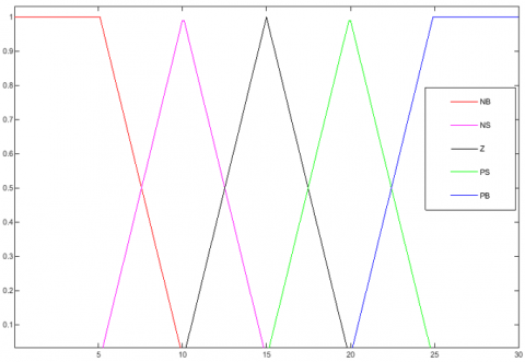
In this case we define fuzzy sets of error variables at the level of glucose in the blood by 5 membership function as follows: ((NB(Negative Big ), NS (Negative Small), Z(Zero), PS(Positive Small), PB(positive Big)), and the membership function for the error rate, the blood glucose level by 5 membership functions as follows: (( NB(Negative Big), NS (Negative Small), Z(Zero), PS(Positive Small), PB(positive Big)), and the membership function for output through 5 membership functions as follows: ((NB(Negative Big), NS (Negative Small), Z(Zero), PS(Positive Small), PB(positive Big)), as shown in Figure 3 (a, b, c), As for the rules, they are represented In the Table 4.
8.2 Discussing fuzzy logic results
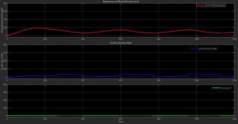
In this part, the control of blood glucose level is simulated by placing a valve that controls the insulin infusion controlled by the fuzzy logic controller, this simulation was performed for a patient 1 with diabetes type 1 based on the parameter value in Table 2. And put turbulence at value D (t)=0.5 e-0.05t At the Time value (80 min) and we kept the insulin value at a constant value of u=15[mU/L].
Through the responses shown in Figure 6; and the results recorded in Table 5, we note that there is a value of less than 120 mg / dL for glucose concentration and we also noticed that there is a too large overshoot and slow responses and the stability was a somewhat late.
After we applied the closed loop system and changed us in the Inputs to the fuzzy logic controller and changed us in the rules, there was a good response and stability at the value 94.5 mg/dl, and that there is good control in the level of glucose in the blood, after it increase to the value 300 mg/dl, which is a very large value, it stays at the value 94.5 mg/dl by controlling it from The valve opening and through fuzzy logic controller and this difference we noticed in Figure 7.
Finally, we can say that the system of closed loop and valve controlled by the fuzzy logic controller provided more satisfactory and positive results and values for controlling the level of glucose in the blood at any desired level, and these differences lie through our comparison with the results of previous studies in Ref. [15].
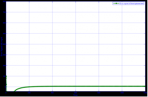
Figure 8 shows the value of the error resulting from the difference between the reference value And the Blood Glucose Level, as it is rounded to the value 0, which indicates that the ٍValve Opening has a major role in reducing the glucose value to the desired level.
Table 3. Comparison of performances of the fifth algorithms for the blood glucose concentration
|
Criteria |
Kp |
Ki |
Kd |
Lamda (λ) |
Mu (u) |
Max overshoot (%) |
Rise time |
Settling time (%) |
Fitness function values |
|
|
PSO |
IAE |
151.0431 |
177.3066 |
157.2816 |
0.95385 |
0.17157 |
1.6157 |
8.0904 |
9.9107 |
1.0331 |
|
ISE |
103.1063 |
198.2578 |
148.5963 |
0.98045 |
0.23478 |
1.5082 |
8.0803 |
9.8983 |
1.0004 |
|
|
IWO |
IAE |
151.1334 |
191.4142 |
109.1934 |
0.99304 |
0.096434 |
1.4785 |
8.0789 |
9.8966 |
1.0304 |
|
ISE |
163.7023 |
195.391 |
194.6926 |
0.96661 |
0.067344 |
1.4041 |
8.0814 |
9.8958 |
1.0003 |
|
|
BAT |
IAE |
22.9603 |
93.612 |
68.3189 |
0.96211 |
0.43797 |
3.3938 |
8.1848 |
23.0587 |
1.0707 |
|
ISE |
22.9603 |
93.612 |
68.3189 |
0.96211 |
0.43797 |
3.3938 |
8.1848 |
23.0587 |
1.0018 |
|
|
ACO |
IAE |
8.9573 |
8.8777 |
3.9361 |
0.67546 |
0.25221 |
16.0469 |
12.7230 |
55.1983 |
1.6571 |
|
ISE |
2.613 |
8.9336 |
9.7206 |
0.9940 |
0.34679 |
19.9101 |
10.8963 |
61.4656 |
1.0802 |
|
|
GA |
IAE |
3.7763 |
9.5156 |
7.424 |
0.88709 |
0.5989 |
19.9746 |
11.4077 |
52.6549 |
1.6242 |
|
ISE |
9.5811 |
9.8506 |
5.3472 |
0.90598 |
0.47665 |
18.4961 |
11.1169 |
50.6076 |
1.0762 |
|
In this section, tables and figures are presented to illustrate the effectiveness of these algorithms. To make a comparison of these algorithms. performances of the fifth Algorithms for the Blood Glucose Concentration are given in Table 3; Rules for member ship function in Table 4; Responses of blood Glucose with ISE fitness function in Figure 4; Responses of blood Glucose with IAE fitness function in Figure 5; Fuzzy Logic Controller for blood Glucose and insulin infusion Rate without feed-back in Figure 6 And Fuzzy Logic Controller for blood Glucose And insulin infusion Rate with feed-back in Figure 7.
Table 4. Rules for inference system
|
Error of blood Glucose and References e(k) |
|
|||||
|
PB |
PS |
Z |
NS |
NB |
|
|
|
Z |
NS |
NB |
NB |
NB |
NB |
Error of changing blood Glucose and References e(k) |
|
PS |
Z |
NS |
NB |
NB |
NS |
|
|
PB |
PS |
Z |
NS |
NB |
Z |
|
|
PB |
PB |
PS |
Z |
NS |
PS |
|
|
PB |
PB |
PB |
PS |
Z |
PB |
|
Table 5. Fuzzy logic controller for glucose level concentration
|
|
Glucose Level Concentration |
Stable state of glucose |
|
Fuzzy Logic Controller without feedback |
200 mg/dl |
Unstable<170 mg/dl |
|
Fuzzy Logic Controller with feedback |
400 mg/dl |
94.5 mg/dl |
a. Diagram of fuzzy logic controller without feed back for BGC
b. Diagram of fuzzy logic controller with feed back
Figure 1. Block diagram of fuzzy logic controller
Figure 2. Responses of test Bergman
a. Input membership function of error glucose concentration [mg/dl]
b. Input membership function of rate of error glucose concentration [mg/dl]
c. Output membership function
Figure 3. Input and output of member functions of fuzzy logic controller
Figure 4. Responses of blood glucose with ISE fitness function
Figure 5. Responses of blood glucose with IAE fitness function
Figure 6. Fuzzy logic controller for blood glucose and insulin infusion rate without feed-back
Figure 7. Fuzzy logic controller for blood glucose and insulin infusion rate with feed-back
Figure 8. The error signal between the reference value and the blood glucose level
In this paper, a robust control tool is designed to regulate blood glucose level of type 1 diabetes patients. Bergmann model was used to simulate the relationship between insulin and glucose and the effect of insulin infusion and control of glucose concentration in the blood as an artificial pancreas and this is what we demonstrated through simulation.
After that, five modern technical methods were used to solve optimization problems, one of which is the Particle Swarm Optimization (PSO), The bat optimization algorithm (BA), Invasive Weed Optimization (IWO), Ant Colony Optimization (ACO) and technology Genetic Algorithm (GA) to adjust the parameters of the proposed control unit which is FO-PID by reducing the cost function subject to constraints, reducing error and speed of implementation. Methods are strength in problem solving and in finding better performance, but it became clear to us that the IWO and PSO method is a better method of improvement than other methods for solving multi-purpose problems, and it is easy to implement and computationally effective methods. For IWO, it was better compared to PSO, even if with a slight difference in terms of reducing error and cost function, on the other hand, we concluded that the proposed FO-PID Control unit with fractional order effectively affected blood glucose level with good performance.
As for the valve control and the fuzzy logic Controller, this control unit presented very positive results in terms of reducing error, stability at a value of 95.11 mg/dl and good control of insulin pumping.
[1] Friis-Jensen, E. (2007). Modeling and simulation of glucose-insulin metabolism. In Congress Lyngby.
[2] Sharma, R., Mohanty, S., Basu, A. (2016). Tuning of digital PID controller for blood glucose level of diabetic patient. In 2016 IEEE International Conference on Recent Trends in Electronics, Information &Communication Technology (RTEICT), pp. 332-336. https://doi.org/10.1109/RTEICT.2016.7807837
[3] World Health Organization (2020). https://www.who.int/health-topics/diabetes#tab=tab_1
[4] Sivaramakrishnan, N., Lakshmanaprabu, S.K., Muvvala, M.V. (2017). Optimal Model Based Control for Blood Glucose Insulin System Using Continuous Glucose Monitoring. Journal of Pharmaceutical Sciences and Research, 9(4): 465.
[5] Farman, M., Saleem, M.U., Ahmad, M.O., Tabassum, M.F., Meraj, M.A. (2016). Exploring mathematical models for the treatment of type-I diabetes. Science International, 28(2): 795-798.
[6] Loutseiko, M., Voskanyan, G., Keenan, D.B., Steil, G.M. (2011). Closed-loop insulin delivery utilizing pole placement to compensate for delays in subcutaneous insulin delivery. Journal of Diabetes Science and Technology, 5(6): 1342-1351. https://doi.org/10.1177/193229681100500605
[7] Heydarinejad, H., Delavari, H., Baleanu, D. (2019). Fuzzy type-2 fractional Backstepping blood glucose control based on sliding mode observer. International Journal of Dynamics and Control, 7(1): 341-354. https://doi.org/10.1007/s40435-018-0445-8
[8] Ridha, T.M.M., Kadhum, M.Q., Mahdi, S.M. (2011). Back stepping-based-PID-controller designed for an artificial pancreas model. Al-Khwarizmi Engineering Journal, 7(4): 54-60.
[9] Parsa, N.T., Vali, A.R., Ghasemi, R. (2014). Back stepping sliding mode control of blood glucose for type I diabetes. World Academy of Science, Engineering and Technology, International Journal of Medical, Health, Biomedical, Bioengineering and Pharmaceutical Engineering, 8(11). https://doi.org/10.5281/ZENODO.1096773
[10] Karam, E.H., Jadoo, E.H. (2020). Design modified robust linear compensator of blood glucose for type I diabetes based on neural network and PSO algorithm. Control Science and Engineering, 3(2): 29-36. https://doi.org/10.11648/j.cse.20190302.12
[11] Kovács, L., Paláncz, B., Endre, B., Benyó, B.I., Benyó, Z. (2010). Robust Control Algorithms for Blood-Glucose Control using Mathematica.
[12] Quesada, L.F., Rojas, J.D., Arrieta, O., Vilanova, R. (2019). Open-source low-cost Hardware-in-the-loop simulation platform for testing control strategies for artificial pancreas research. IFAC-PapersOnLine, 52(1): 275-280. https://doi.org/10.1016/j.ifacol.2019.06.074
[13] Soylu, S., Danisman, K. (2016). Comparison of PID based control algorithms for daily blood glucose control. In ASET 2016 International Conference on Electrical Engineering and Electronics, pp. 16-17. https://doi.org/10.11159/eee16.130
[14] Malik, S.F.J.M. (2018). Particle swarm optimisation based blood glucose control in type1 diabetes. Doctoral dissertation, Kauno technologijos universitetas.
[15] Almeida, R., Tavares, D., Torres, D.F. (2019). The Variable-Order Fractional Calculus of Variations. Springer International Publishing. https://doi.org/10.1007/978-3-319-94006-9
[16] Goharimanesh, M., Lashkaripour, A., Abouei Mehrizi, A. (2015). Fractional order PID controller for diabetes patients. Journal of Computational Applied Mechanics, 46(1): 69-76. https://doi.org/10.22059/JCAMECH.2015.53395
[17] Milici, C., Drăgănescu, G., Machado, J.T. (2019). Introduction to fractional differential equations (Vol. 25). Springer. https://doi.org/10.1007/978-3-030-00895-6
[18] Monje, C.A., Chen, Y., Vinagre, B.M., Xue, D., Feliu-Batlle, V. (2010). Fractional-order systems and controls: fundamentals and applications. Springer Science & Business Media. https://doi.org/10.1007/978-1-84996-335-0
[19] Vakilia, S., ToosianShandizb, H. (2019). Fractional order glucose insulin system using fractional back-stepping sliding mode control. Int. J. Nonlinear Anal. Appl, 10(2): 1-10. https://doi.org/10.22075/IJNAA.2019.4067
[20] Nath, A., Deb, D., Dey, R., Das, S. (2018). Blood glucose regulation in type 1 diabetic patients: An adaptive parametric compensation control-based approach. IET Systems Biology, 12(5): 219-225. https://doi.org/10.1049/iet-syb.2017.0093
[21] Tejado, I., Vinagre, B.M., Traver, J.E., Prieto-Arranz, J., Nuevo-Gallardo, C. (2019). Back to basics: Meaning of the parameters of fractional order PID controllers. Mathematics, 7(6): 530. https://doi.org/10.3390/math7060530
[22] Kramer, O. (2017). Genetic algorithm essentials (Vol. 679). Springer. https://doi.org/10.1007/978-3-319-52156-5
[23] Doyle, F.J., Huyett, L.M., Lee, J.B., Zisser, H.C., Dassau, E. (2014). Closed-loop artificial pancreas systems: engineering the algorithms. Diabetes Care, 37(5): 1191-1197. https://doi.org/10.2337/dc13-2108
[24] Baker, L., Maley, J.H., Arévalo, A., DeMichele, F., Mateo-Collado, R., Finkelstein, S., Celi, L.A. (2020). Real-world characterization of blood glucose control and insulin use in the intensive care unit. Scientific Reports, 10(1): 1-10. https://doi.org/10.1038/s41598-020-67864-z
[25] Ebrahimi, N., Ozgoli, S., Ramezani, A. (2020). Model free sliding mode controller for blood glucose control: Towards artificial pancreas without need to mathematical model of the system. Computer Methods and Programs in Biomedicine, 195: 105663. https://doi.org/10.1016/j.cmpb.2020.105663
[26] Bertachi, A., Ramkissoon, C.M., Bondia, J., Vehí, J. (2018). Automated blood glucose control in type 1 diabetes: A review of progress and challenges. Endocrinología, Diabetes y Nutrición (English ed.), 65(3): 172-181. https://doi.org/10.1016/j.endien.2018.03.001
[27] Babar, S.A., Rana, I.A., Mughal, I.S., Khan, S.A. (2021). Terminal synergetic and state feedback linearization based controllers for artificial pancreas in type 1 diabetic patients. IEEE Access, 9: 28012-28019. https://doi.org/10.1109/ACCESS.2021.3057365
[28] Bonyadi, M.R., Michalewicz, Z. (2017). Particle swarm optimization for single objective continuous space problems: A review. https://doi.org/10.1162/EVCO_r_00180
[29] Clerc, M. (2010). Particle Swarm Optimization (Vol. 93). John Wiley & Sons.
[30] Mehmood, S., Ahmad, I., Arif, H., Ammara, U.E., Majeed, A. (2020). Artificial pancreas control strategies used for type 1 diabetes control and treatment: A comprehensive analysis. Applied System Innovation, 3(3): 31. https://doi.org/10.3390/asi3030031
[31] Belmon, A.P., Auxillia, J. (2020). An adaptive technique based blood glucose control in type‐1 diabetes mellitus patients. International Journal for Numerical Methods in Biomedical Engineering, 36(8): e3371. https://doi.org/10.1002/cnm.3371
[32] Xie, J., Zhou, Y., Chen, H. (2013). A novel bat algorithm based on differential operator and Lévy flights trajectory. Computational Intelligence and Neuroscience. https://doi.org/10.1155/2013/453812
[33] Ma, X.X., Wang, J.S. (2018). Optimized parameter settings of binary bat algorithm for solving function optimization problems. Journal of Electrical and Computer Engineering. https://doi.org/10.1155/2018/3847951
[34] Goli, A., Zare, H.K., Tavakkoli-Moghaddam, R., Sadeghieh, A. (2019). Application of robust optimization for a product portfolio problem using an invasive weed optimization algorithm. Numerical Algebra, Control & Optimization, 9(2): 187. https://doi.org/10.3934/naco.2019014
[35] Misaghi, M., Yaghoobi, M. (2019). Improved invasive weed optimization algorithm (IWO) based on chaos theory for optimal design of PID controller. Journal of Computational Design and Engineering, 6(3): 284-295. https://doi.org/10.1016/j.jcde.2019.01.001
[36] Ramprasad, Y., Rangaiah, G.P., Lakshminarayanan, S. (2004). Robust PID controller for blood glucose regulation in type I diabetics. Industrial & Engineering Chemistry Research, 43(26): 8257-8268. https://doi.org/10.1021/ie049546a
[37] Kirchsteiger, H., Jørgensen, J.B., RenardE, D.R.L. (2016). Prediction methods for blood glucose concentration, p. 265. Switzerland: Springer International Pulblishing. https://doi.org/10.1007/978-3-319-25913-0
[38] Anastassiou, G.A., Argyros, I.K. (2016). Intelligent numerical methods: Applications to fractional calculus. Springer International Publishing. https://doi.org/10.1007/978-3-319-26721-0
[39] Chee, F., Fernando, T. (2007). Closed-loop control of blood glucose (Vol. 368). Springer.
[40] Ibbini, M.S., Masadeh, M.A., Bani Amer, M.M. (2004). A semiclosed-loop optimal control system for blood glucose level in diabetics. Journal of Medical Engineering & Technology, 28(5): 189-196. https://doi.org/10.1080/03091900410001662332
[41] Boldisor, C., Coman, S. (2015). Simulations of a Model-Based Fuzzy Control System for Glycemic Control in Diabetes. Bulletin of the Transilvania University of Brasov. Engineering Sciences. Series I, 8(2): 93.
[42] Chiranjeevi, S.B. (2016). Implementation of fractional order PID controller for an AVR system using GA and ACO optimization techniques. IFAC-PapersOnLine, 49(1): 456-461. https://doi.org/10.1016/j.ifacol.2016.03.096