Hayam G. Wahdan* | Hisham M. Abdelslam | Sally S. Kassem
© 2021 IIETA. This article is published by IIETA and is licensed under the CC BY 4.0 license (http://creativecommons.org/licenses/by/4.0/).
OPEN ACCESS
Modularity concepts play an important role in the process of developing new complex products. Modularization involves dividing a product into a set of modules - each of which consisting of a set of components - that are interdependent in the same cluster and independent between clusters. During this process, a product can be represented using a Design Structure Matrix (DSM). A DSM acts as a tool for system analysis to provide clear visualization of product elements. In addition, DSM, shows the interactions between these product elements. This paper aims to propose an efficient optimization algorithm that dynamically divides a DSM into an optimal number and size of clusters in a way that minimizes total coordination cost; the interactions inside clusters (modules) and interactions between clusters. Given problem complexity, five metaheuristic optimization algorithms are proposed and tested to solve it; these algorithms are used to determine: (1) the optimal clusters’ number within a DSM, and (2) the optimal components assignment clusters to minimize the total coordination cost. The five used metaheuristics are: Cuckoo Search, Modified Cuckoo Search, Particle Swarm Optimization, Simulated Annealing, and Gravitational Search Algorithm. Eighty problems with different properties are generated and used to examine the proposed algorithms for effectiveness and efficiency. Extensive comparisons are conducted and analyzed. Cuckoo Search is outperforming the other four algorithms.
modular design, Design Structure Matrix, Cuckoo Search, Particle Swarm Optimization, Simulated Annealing, Gravitational Search Algorithm
Modular design has a significant impact on product development processes that respond to market trends requiring large varieties within small production processes [1]. Modularity is an important method to break down large systems into smaller modules for easier management of such large systems. The modules are interdependent in the same module and independent between different modules. Modular design involves clustering different components forming a product to create modules which are effective and useful for production. Effective product modularity acquires more importance when similar modules are used in different products [2]. A desirable product architecture is an architecture that partitions a product into modules such that, some modules can be updated on regular cycles of time, others can be changed to generate various type of products, others can be deleted without affecting the product function, and some other modules might be swapped to offer additional functionality [3].
Modularity has an impact on profit and sustainability. Concerning manufacturers, a modular product has modules that can be replaced with newly developed modules, without the need to develop or manufacture entirely new products. Concerning customers, they can upgrade their products by replacing existing modules with new upgraded ones without the need to dispose of the product. This leads to reducing total waste since the entire product will not be disposed [4].
Design Structure Matrix (DSM) is a well-recognized tool that assists in the analysis, as well as, management of large and complex systems [5]. Also, it is a product representation tool used to model, visualize, and analyze dependencies between the elements of a system, and recommends actions for the improvement or formation of a DSM to represent a system. A product can be represented by a DSM containing a list of the product’s components. Product’s DSM also provides information exchange and dependency relationships among these components [6]. Transformation an initial DSM to functional blocks of components is a process known as DSM clustering; the clustering process creates modules which are effective and useful for the company [7].
Within such context, this paper aims to propose an efficient algorithm that divides a DSM into clusters based on minimizing the total coordination cost as the objective function. The total coordination cost is a term introduced by Gutierrez (1998) to quantify the summation of interactions inside clusters (IntraClusterCost) and interactions between clusters (ExtraClustercost) [8]. To propose such efficient algorithm, a number of metaheuristic algorithms, available in the literature, are considered. The algorithms are tailored to solve the problem of dividing a DSM into clusters with the objective of minimizing the total coordination cost. In this paper, five metaheuristic algorisms are used to determine: (1) the optimal number of clusters of DSM, and (2) the optimal components assignment to clusters such that the total coordination cost is minimized. The five metaheuristic algorithms utilized in this work are:
1-Cuckoo Search (CS)
2- Modified Cuckoo Search (MCS)
3- Particle Swarm Optimization (PSO)
4- Simulated Annealing (SA)
5- Gravitational Search Algorithm (GSA)
Comprehensive comparisons are conducted between the results obtained using the five metaheuristic algorithms. The output of the comparisons is a recommendation on the efficient algorithm to solve the problem presented in this research.
To the best of our knowledge, this is the first time to use these metaheuristic algorithms with cost minimization as the objective function in solving product design problem under modularity while having dynamic number of clusters.
Following the introduction, the rest of the paper is structured as follows: Section 2 provides a brief introduction about DSM, followed by a review of related literature in Section 3. Problem definition and proposed solution algorithms are provided in Sections 4 and 5, respectively. Section 6 includes numerical experimentation and analysis of the algorithms and, finally, the paper conclusion and points for future research are provided in Section 7.
The Design Structure Matrix (DSM) is a system analysis tool which provides a compact and clear representation of a complex large system. It determines the interaction/interdependencies/interfaces between elements forming a system. DSM allows feedback, in addition to cyclic dependencies. This is one of the most important features of DSMs since many engineering applications possess that cyclic property [9].
DSM is a square matrix of size n, is the number of elements of the system. Figure 1 shows an example of a DSM of size 7. Elements names are written on the first raw and the first column of the matrix in the same order. An entry of 1 or x in the matrix means that the correspond elements i j (rowi, columnj) are dependent on each other [10]. A DSM is established for each product, and can be analyzed to identify modules, such process is known as clustering. DSM clustering aims at finding clustering arrangements where modules interact minimally with each other, and at the same time, components belonging to the same module maximally interact with each other [6]. For example, Figure 1(a) shows the original DSM without clustering, Figure 1(b) shows the DSM after clustering where most interactions are contained in two modules, namely, {A, F, E} and {D, B, C, G}. Figure 1(b) also shows that three interactions do not belong to any specific module.
Figure 1. Example of Design Structure Matrix [11]
Cuckoo Search clustering algorithm is used to find the optimal number of clusters and the optimal assignment of components to clusters with total coordination cost as an objective [6, 9]. Genetic clustering is proposed with Minimum Description Length measure. a new assumption is added to minimize the total execution time. The proposed algorithm is tested on four case studies [7]. mathematical model was developed by Gutierrez [8], this model minimizes the coordination cost [8] with fixed number of clusters. A Genetic Algorithm is used to find optimal arrangement of elements within DSM which optimize the minimum description length (MDL) [11].
Eppingeret et al. introduced the idea of minimizing interactions between modules, while maximizing interactions within modules in a DSM [12]. Idicula proposed a stochastic clustering algorithm for DSM clustering [13]. Thebeau developed a stochastic hill climbing algorithm to cluster DSM with the objective function of cost minimization [14].
A new method is developed to define the difference between designing modular systems and integrative systems [15]. The study is focused on the specification of modules, modules architecture, and their interfaces.
To obtain better output from a clustering algorithm, a method known as conceptual module generation phase can be employed [16]. Liang [17] developed a model known as group decomposition model. The proposed model decomposes a complex set of activities into simpler ones. The DSM is used as a system simplification tool. The clustering algorithm employed is K-means algorithm [17]. Li [18] proposed an integrated tool that addresses problems in matrix-based decomposition [18]. Four DSM types are provided with their corresponding application in engineering design, as well as, in concurrent engineering. Various techniques dealing with DSM partitioning, taring, banding, and clustering are proposed [19]. A modularization scheme based on functional modeling is proposed and K-means is used for clustering [20]. Neural networks algorithms and DSMs have been utilized to cluster DSM components with the objective function of clustering efficiency; however, the algorithm requires a predetermined number of clusters [21]. Borjesson and Hölttä [22] develop an algorithm named Idicula-Gutierrez-Thebeau Algorithm (IGTA) for clustering DSM. An improved algorithm, named IGTA-plus, is proposed. IGTA-plus provide significant improvement when compared with IGTA. Recorded improvements are in terms of computational time and solution quality [22].
Yang et al. [23] developed a systematic clustering algorithm for organizational DSM. The algorithm evaluates clustering structures based on the strength of interaction.
Another novel approach for product design is introduced by integrating the sequence structure planning of assembly and disassembly of a product [24].
A hybrid approach is developed, based on multidimensional scaling (MDS) and clustering methods. This approach is applied on DSM to provide product architecting [25]. A new practical method is proposed by Sakao et al. to support designers in creating service modules by extending the DSM [26]. research focused on the answering the questions, how modularity used in product design, how it is helped in product Varity and how modularity increased the organization performance [27], Finally Non-dominated Cuckoo Search is proposed to maximize Sustainability through DSM, This multi objective optimization technique wants to find s set of Pareto optimal solutions; each solution represents the structure of modules and the number of modules in the product which optimize functionality and sustainability objectives. The problem has set of conflicting objectives, product functionality objective, labor time, environmental impact and labor cost. [28].
The reviewed literature on product design using DSM as a system analysis tool revealed the existence of several points of view to cluster the DSM for modularity. One major difference between those points of view is the objective of clustering. Another difference is in the solution technique. Considering the objective of clustering, Minimal Description Length (MDL) is one of the objectives [11]. Another objective is Minimizing the total coordination cost, which is recognized as one of the most widely targeted objectives [14]. Clustering Efficiency (CE) index with static number of clusters is also among the considered objectives in the literature [21]. As for the solution technique for solving the problem, several techniques exist in the literature, for example: Genetic Algorithm [11], stochastic hill-climbing algorithm [14], and neural networks [21].
To the best of our knowledge, this research is the first one to use the five previously mentioned metaheuristic algorithms with cost minimization as the objective function in solving product design problem under modularity with dynamic number of clusters.
Consider the DSM shown in Figure 1, if component i is dependent on component j, then the matrix element i j (rowi, columnj) contains “1” or “x” otherwise it contains “0” or remains empty. The objective is to cluster these components in such a way that minimizes the total coordination cost. Accordingly, two sets of decisions are to be considered; (1) the number of clusters will be formed, and (2) the optimal assignment of components in each cluster.
For a given DSM, the total coordination cost consists of two parts; IntraClusterCost and ExtraClusterCost as provided by equations 1 and 2, respectively. If interaction DSMik belongs to cluster j then IntraClusterCost is to be calculated, otherwise ExtraClusterCost is to be calculated. The total cost is the summation of IntraClusterCost and ExtraClusterCost as shown in Eq. (3) and mentioned by Borjesson & ltta-Otto [29].
$\begin{aligned} \text { intraClusterCost } &=\sum_{i, k \in \text { Clusterj }}(\text { DSMik }+\text { DSMki }) \\ * & \sum_{j=1}^{\text {ncluster }}(\text { ClusterSize } j)^{\text {powcc }} \end{aligned}$ (1)
ExtraClustercost $=\sum_{i, k \notin \text { clusterj }}$ (DSMik
$+D S M k i)$ DSMSize $^{\text {powco }}$
$j=1 \ldots$ ncluster (2)
where, DSMik is the relation between elements i and k, DSMSize is the number of elements (rows) in the matrix, powcc is a value utilized to penalize clusters’ sizes, and ncluster is the total number of clusters. Clustersize(j) is the number of elements within cluster j.
Total coordination Cost = IntraClusterCost + ExtraClusterCost (3)
The problem under consideration involves one key constraint, which is: each element must be assigned to a single cluster; i.e., overlapping between clusters is prohibited. Prohibiting overlapping, or multi-cluster elements is necessary since elements existing in several clusters force these common clusters to have interactions between each other on multi-levels. These interacting clusters reduce or even diminish the usefulness and efficiency of the clustering process.
Metaheuristic optimization algorithms are general iterative algorithms capable of solving combinatorial optimization problems. These algorithms are stochastic in manner. They simulate the behavior of particles. Metaheuristic algorithms try to find optimal or near optimal solutions for complex problems [30] To solve the problem in this research, five metaheuristic algorithms are utilized. Four of the selected algorithms represent a population-based optimization method, and one algorithm represents a trajectory optimization method. The selected algorithms are Cuckoo Search (CS), Modified Cuckoo Search (MCS), Particle Swarm Optimization (PSO), Gravitational Search Algorithm (GSA), and Simulated Annealing (SA). In the following subsections, a brief description of the algorithms is given, along with a pseudo code to provide easy implementation to the problem under consideration.
5.1 Cuckoo Search (CS)
The Cuckoo Search (CS) algorithm was proposed by Yang and Deb [31]. The algorithm simulates the behavior of cuckoo birds to explore the solution space for an optimum or near optimum solution. CS is inspired from the behavior of some brood parasite cuckoo species that lay their eggs in the nests of host birds of other species. Brood parasite cuckoos distribute their eggs among several different nests. Their aim is to escape the parental investment in raising their offspring, and to minimize the risk of their egg loss [31].
One of the significant advantages of CS is its efficiency that has been proven using a considerable number of benchmark studies. When comparing results with other metaheuristic algorithms, CS performed better. Another advantage of CS compared to other metaheuristic algorithms is its simplicity, since it requires setting only two parameters. This feature simplifies the time and effort needed to adjust and fine tune the algorithm’s parameter settings [32].
In CS algorithm, an egg represents a solution. Initial solutions are randomly generated. Xit is solution i in generation t. Xit+1 is obtained using a levy flight using equation 4. A levy flight is a random walk with step lengths that follow a heavy tailed probability distribution given in Eq. (5). Random walks through Lévy flights experience longer step lengths on the long run, and hence are efficient in exploring search spaces.
$\mathrm{X}_{\mathrm{i}}^{\mathrm{t}+1}=\mathrm{X}_{\mathrm{i}}^{\mathrm{t}}+\alpha \oplus \operatorname{Levy}(\lambda)$ (4)
where, α is a number greater than zero that denotes the step size, $\oplus$ product denotes entry-wise multiplications.
Levy ∼ u = t −λ, (1 < λ ≤ 3) (5)
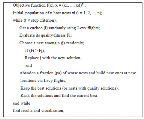
The main steps of the CS algorithm are given in the pseudo code in Figure 2.
Figure 2. Pseudo code of CS [33]
5.2 Modified Cuckoo Search (MCS)
A Modified Cuckoo Search algorithm was provided by Walton et al. [33] with the same structure of original Cuckoo Search maintained but with two modifications. The first modification is changing the size of the Levy flight step size α. In CS, α is set to the value of 1, and hence has a constant value at all generations. In MCS, the value of α decrease as the number of generations increases. This modification leads to a more localized search as the individuals, or the eggs, get closer to the solution. The second modification is the information exchange among the eggs, aiming to speed convergence of the solution. In CS, there is no information exchange among individuals, and hence, searches are performed independently.
In MCS, a fraction of the eggs with the best fitness are categorized as a group of top eggs. Two eggs are randomly chosen from the group of top eggs. A new egg is then generated on the line connecting the two chosen top eggs. The new egg is located closer to the egg with the best fitness. The distance of the new egg along the line is calculated using the inverse of the golden ratio ᶲ =(1+√5)/2. If the two chosen top eggs have the same fitness value, then the new egg is placed at the midpoint. If the same egg is chosen twice, a local Levy flight search is performed from the randomly picked nest with step size α = A/G2 [34].
5.3 Particle Swarm Optimization (PSO)
Figure 3. Pseudo code of PSO [35]
The PSO algorithm was first introduced by Kennedy and Eberhart [36]. The algorithm was inspired by mimicking the social behavior of flocks of birds or schools of fishes. A flock of birds or a school of fishes has a leader. The leader guides the movement of all individuals of the swarm. The movement of every individual depends of the leader’s knowledge [36]. The main steps of the PSO algorithm are summarized in the pseudo code in Figure 3.
5.4 Gravitational Search Algorithm (GSA)
The GSA was first proposed by Rashedi et al. [37] as a nature-inspired algorithm. The algorithm is population-based, where Newton’s laws of gravity and motion are considered to solve complex optimization problems. GSA is based on the law of gravity and mass interactions. The algorithm requires a set of search agents that interact with each other through gravity force [37].
Steps of the GSA algorithm are summarized in the pseudo code in Figure 4.
Figure 4. Pseudo code of GSA [38]
5.5 Simulated Annealing (SA)
The SA algorithm was proposed in 1982 by Kirkpatric et al. [39]. SA is a probabilistic local search technique used to find an optimum or near optimum solutions for large combinatorial optimization problems. SA is best used when the search space is discrete. Simulated Annealing imitates the annealing process of metals. The algorithm explores the solution space using neighborhood search methods. Worse solutions are accepted with low probabilities to avoid being trapped in local optima [39]. Basic steps of the SA algorithm are summarized in the pseudo code in Figure 5
Figure 5. Pseudo code of SA [40]
5.6 Implementation
5.6.1 Solution representation
Solution representation of the problem is a vector of length that is equal to the number of elements of the DSM. Each value in the vector is an integer between 1 and the number of clusters, as shown in Figure 6. Figure 6 illustrates a vector of size 7. The vector represents a solution for an original DSM consisting of 7 elements. The solution presented in Figure 6 means that cluster 1 contains elements 1 and 7, cluster 2 contains elements 2, 3, and 4, and cluster 3 contains elements 5 and 6. The presented solution representation ensures avoiding multi-clustering; in other words, each element will be assigned to exactly one cluster. The solution procedure starts with a number of clusters that is equal to the number of elements available within the DSM. Hence, the solution procedure starts with the maximum possible number of clusters. The next step is to reform sets of clusters to obtain the optimum number of clusters with the corresponding elements in each cluster.
Figure 6. Solution representation vector
In this work, five algorithms are proposed to solve the problem in hand. Four of the proposed algorithms (CS, MCS, PSO and GSA) are present in the literature to solve continuous optimization problems. The problem presented in this work is discrete in nature, and hence, the proposed algorithm requires a process of discretization. Several methods are available in the literature to perform discretization. Among the known discretization methods is the random key technique, where continuous values are transformed into discrete integer values [41]. Another method is the smallest position value (SPV) [42]. A different technique available in the literature is the nearest integer (NI) method. In this method, a continuous valueis trasnformed to thenearestinteger value by simply rounding, trancatingup, or trancatingdown [43].
SPV and random key methods do not permit the repetition of integer values in the solution. Solving the problem presented in this research necessarily requires repeating some integer values. Hence, SPV and random key methods cannot be used to solve the problem in hand. The nearest integer method, on the other hand, allows the repetition of integer values in a solution, and therefore, the nearest integer discretization technique is chosen to solve the problem in this research.
When using CS and MCS to cluster a DSM, the algorithm begins with generating several nests. A nest consists of a vector having a length that is equal to the number of elements of the DSM to be clustered. Entries of vectors are randomly generated uniformly between the upper limit and lower limit. Then, these entries are transformed into integer values using the nearest integer method. Vectors represent solutions that require evaluation. Therefore, each vector is sent to the evaluation function. The evaluation function calculates the corresponding total coordination cost, conducts comparisons and performs updates using Levy flight and the probability of discovery (pa), details are available in Section 5.1 and Section 5.2.
In PSO, the algorithm begins with generating several particles. A particle consists of a vector having a length that is equal to the number of elements of the DSM to be clustered. Entries of vectors are randomly generated uniformly between the upper limit and lower limit. Then, these entries are transformed into integer values using the nearest integer method. Vectors represent solutions that require evaluation. Therefore, each vector is sent to the evaluation function. The evaluation function calculates the corresponding total coordination cost, and generates a new solution using a new position and a new velocity. Details are given in Section 5.3.
Finally, in GSA, the process starts with a set of objects. The fitness function is evaluated, mass and acceleration are calculated, and the velocity and position are updated to generate a new solution Details are given in Section 5.4.
Regarding SA, the solution is a vector of length that equals to the number of elements in the DSM. This vector contains integer numbers whose values are between lower and upper limits. The vector represents the current solution. A new solution is updated by generating a neighbor solution, then old and new solutions are compared. Details are given in Section 5.5.
5.6.2 Solution evaluation
Clustering a DSM requires minimizing the total coordination cost which is based on IntraClusterCost and ExtraClusterCost. IntraClusterCost is calculated if interaction DSMik belongs to cluster j, otherwise, ExtraClusterCost is calculated. At the beginning of the solution procedure, feasible solutions are randomly generated, and the total coordination cost is calculated. Details of calculating the total coordination cost, IntraClusterCost, and ExtraClusterCost, are given in Section 4. Evaluation of the solution(s) is performed, then the algorithm selects the best obtained solution and a new iteration begins. In this research, five algorithms are used, hence, each algorithm moves to the next solution according to its specific procedure as follows: (1) CS and MCS utilize Levy flight to move the best nests with high quality eggs (solutions) to the following generation, (2) PSO moves to a new position with a different velocity, (3) SA obtain a neighbor solution (4) GSA utilizes a set of agents, each agent has a corresponding position, inertial mass, active gravitational mass, and passive gravitational mass. Gravitational masses and inertia masses are adjusted in each iteration to obtain the new solution, where the heaviest mass represents the best obtained solution. Each of the five algorithms moves from generation to the next till the stopping criteria is reached.
5.6.3 Handling constraints
The five proposed algorithms rely on unconstraint objective function evaluation. The problem considered in this research is a constrained problem. Hence, a constraint handling method is required to solve the problem considered in this research. There are several methods that can be used to handle constraints, one of the simplest and most common methods is using a penalty function. The main idea is to transform a constrained optimization problem to an unconstrained optimization problem by adding a certain value (penalty) to the objective function. This value depends on the amount of violation presented in a certain solution [44].
In the proposed algorithms, a penalty is added to the fitness function according to Eqns. (6) and (7) which guarantee reaching a feasible solution as iterations proceed.
penalty $(\mathrm{x})=\left\{\begin{array}{c}0, \text { if no violation occurs } \\ (\mathrm{C} * \text { iter })^{\alpha} \sum_{\mathrm{j}=1}^{\mathrm{m}} \mathrm{f}_{\mathrm{j}}^{\beta}(\mathrm{x}), \text { otherwise }\end{array}\right.$ (6)
$\operatorname{eval}(x) \\ \quad=\left\{\begin{array}{l}f(x), \quad \text { if } x \in \text { feasible solutions } \\ f(x)+\text { penalty }(x), & \text { otherwise }\end{array}\right.$ (7)
where, f(x) is the fitness function (total coordination Cost), $(C * \text { iter })^{\alpha}$ is to make the constraint violation of the same order of magnitude as the objective function based on iter (iteration number) violation which expands when iterations grow; β is defined as the multiplication of violation which highly leads to feasibility by maximizing violation value which, in turn, encourages the solution to be feasible through differentiating between feasible and non-feasible solutions with a high impact.
This section compares results obtained by the five algorithms in solving the 80 test problems with different dimensions and complexities.
6.1 Test problems
In order to examine the performance of the proposed algorithms, and hence recommend the efficient algorithm, they are applied to a number of test instances. Due to the limited benchmark instances available in this field, 80 DSMs are randomly generated. These matrices contain 1's and 0's. Numbers of Ones which represent the existence of interaction are generated according to specific complexity. These matrices range from size 10 (number of elements in DSM) up to 100, and from complexity 0.2 up to 0.9. Complexity is defined as the ratio between the numbers of actual interactions to the total number of possible interactions in a given DSM. For example, a DSM of size 10 and with 36 interactions among its components will have a complexity of 36/ ((10x10)-10) = 0.4; where the (10*10)-10) is the total number of possible interactions in a given DSM and 36 is actual interactions.
Based on size, these problems are classified to small (10 to 50 elements), and large (60 to 100 elements). Based on complexity, these problems are classified as low complexity (0.2 to 0.5), and high complexity (0.6 and 0.9).
For the sake of comparison in various experiments, each algorithm is set for 30 runs and 1000 iteration in population-based algorithms, and for SA the initial temperature and final temperature are selected to provide the same number of solution evaluations and exploration of the search space as the other algorithms.
6.2 Algorithms’ performance
Algorithms performance are assessed using the following performance measures: mean value of the objective function, standard deviation, best obtained objective function value, which represents the minimum objective function value among the five algorithms, and the percentage of change from mean. The percentage of change from mean is calculated by dividing the difference between mean and best over best obtained multiplied by 100.
The mean value of the objective function represents the solution quality through 30 runs of each algorithm. Standard deviation is used to assess how far the values are spread above and below the mean. Algorithms with low values of standard deviation tend to be more reliable than those with higher standard deviation values. The best objective function value shows the best solution among the five algorithms. The difference between the mean and best solutions of each algorithm shows the deviation of the mean solution of a specific algorithm from the best value among all algorithms. The low value of the difference indicates that the mean is near to the best. The percentage of change from mean shows the deviation percentage of mean solution of a specific algorithm from the best.
Tables (1-a) to (1-j) (included in appendix) show the results obtained after solving the 80 generated problems using the 5 proposed algorithms. The tables show the mean and standard deviation values for 30 runs of each algorithm at different problems' sizes and complexities. For each table, the best obtained objective function value among the 5 algorithms is identified. Comparisons between the 5 algorithms' objective function values are shown as the difference between the best values obtained and each algorithm's mean objective function value. Tables (2-a) to (2-j) (included in appendix A) show the CPU time, in seconds, for each algorithm to obtain the mean objective function value.
Considering the objective function value as a performance measure, the following can be concluded. For small size and low complexity, CS outperforms 3 algorithms (MCS, PSO and SA) in 40% of the cases regarding the mean objective function value, GSA outperforms the 3 algorithms (MCS, PSO and SA) in 40% of the cases regarding the mean objective function value and the remaining 20% of the cases, the best objective function values are obtained from the others algorithms. For small size and high complexity, CS outperforms the 3 algorithms (MCS, PSO and SA) in 50% of the cases regarding the mean objective function value, GSA outperforms the 3 (MCS, PSO and SA) algorithms in 50% of the cases regarding the mean objective function value and the remaining 3 algorithms do not appear in this case. Considering the large size and low and high complexity, CS outperforms the other 4 algorithms in 100% of the cases regarding the mean objective function value.
Another performance measure considered is the mean computational time. The best algorithm is the one that provides the minimum mean computational time. Results show that for small size and low complexity problems, MCS outperforms the other 4 algorithms in 55% of the cases regarding the mean computational time value. In the remaining 45% of the cases, the best mean computational time values are obtained from the 4 algorithms with different percentages. For small size and high complexity, MCS outperforms the other 4 algorithms in 70% of the cases regarding the mean computational time value. In the remaining 30% of the cases, the best mean computational time values are obtained from the 4 algorithms with different percentages. Considering the large size and low complexity, MCS outperforms the other 4 algorithms in 95% of the cases regarding the mean computational time value. Regarding, large size and high complexity MCS outperforms the other 4 algorithms in 100% of the cases regarding the mean computational time value
The MCS records the worst objective function values due to using probability to discover alien (Pa) with a value of 0.5. In the test problems, this leads to ignoring some better solutions due to this limited local search ability. Therefore, the value of (pa) in the range [0.1, 0.4] for many test instances, achieves the required balance between exploration and exploitation. Similarly, PSO got trapped in local minimum. Considering SA, it is noticed that it obtains inferior solutions compared to the other algorithms. This could be due to the nature of the SA procedure providing a single solution every iteration, and hence the ability to explore the entire solution space is less than the other population-based algorithms. Finally, GSA provides solutions near CS in the small scale problems, but in large scale problems, CS is the best. Regarding CPU time MCS provides the minimum mean CPU time in most cases and in most dimensions. This is due to the second modification done on CS.
The Friedman test is a non-parametric method for identifying treatment discrepancies through several attempts. To rank the performance of the used algorithms using Friedman test [45], Table 3 shows the ranking of algorithms based on the results obtained eighty solved problems using the Friedman test. As expected, the CS algorithm is first in the ranking, GSA is coming next, PSO, MCS and SA respectively.
Table 3. Ranking of algorithms based on performance using Friedman's test
|
Algorithms |
CS |
MCS |
PSO |
SA |
GSA |
|
Ranking |
1.28 |
3.79 |
2.54 |
5 |
2.39 |
To find significant differences between the results obtained by the proposed algorithms in solving the 80 test problems, statistical analysis is used. To detect significant differences in the results, Friedman test is employed. When applying Friedman test using the online Friedman calculator, the result is significance at p < 0.05. This means that the results are important.
Table 4 shows the results of the Friedman test. In this table, there is the Chi-Square value with 4 degrees of freedom, and also there is asymptotic significance of the test (p-value) with very close to zero value. Given the close to zero value of the asymptotic significance, the hypothesis is rejected. Therefore, it can be concluded that there is a significant difference in the performance of algorithms.
Table 4. Results of Friedman’s tests based on performance
|
Test method |
Chi-Square |
Degrees of freedom (DF) |
P-value |
Hypothesis |
|
Friedman |
260.98 |
4 |
0.00001 |
rejected |
6.3 Limiting cluster size
While solving the previous problems, it was noticed that the cluster size can go very large and the first and last clusters were of larger size compared to the others clusters. This is because of the upper and lower bound constraint; this constraint forces elements to be assigned in clusters from 1 to the number of elements, which means that if the element is assigned in a cluster outside the upper bound, it is forced to be assigned to the upper limit cluster, the same applies for the lower bound.
To deal with this issue, two strategies are proposed: (1) elements that are assigned in cluster outside the upper and lower bounds are re-assigned to other clusters within the range and not necessary to either the lower or the upper clusters, and (2) a new constraint is introduced to restrict the maximum number of elements in each cluster. This maximum number of elements in the cluster must be less than or equal the square root of the number of elements in DSM, as mentioned by Yan & Feng [4]. This constraint is incorporated within the model through a penalty function (Eq. (6)) and added to the original objective function of the problem. The penalty function forces solutions that violate the constraint to be ignored in subsequent iterations.
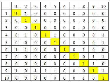
To illustrate the effect of the proposed strategies, consider the original DSM of size 10 and complexity 0.2 shown in Figure 7. Figure 8 Provides DSM after clustering without controlling the size of the clusters. As shown, three clusters are formed and the cluster size is very large, with 5 interactions outside clusters, representing 29% of total interactions, and 71% are included in clusters. This means that the clustering efficiency is 71%. Clustering efficiency is a modularity measure which calculates the percentage of interactions inside clusters with respect to total number of interactions.
Figure 9 shows a clustered DSM after controlling the size of the clusters. Four clusters are formed, which represents the best number of clusters. Elements 1, 2, and 6 are in cluster number 1, element 3 is in cluster number 2 and so on. Nine interactions remain outside clusters, which represents 53% of the total interactions, 47% are included in clusters. This means that the clustering efficiency is 47%.
Figure 7. Original DSM
Figure 8. Clustered DSM without limiting cluster size
Figure 9. Clustered DSM with limited cluster size
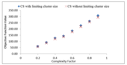
Figures 10 to 14 show the effect of limiting cluster size on results obtained by CS algorithm on some test problems. The figures show that the objective function value is increased after limiting the size of a cluster. This increase happened for all problems’ dimensions and complexities. On the other hand, limiting the size of a cluster is important in modular product design. The smaller the modules, the more practical they are when they need to be replaced or upgraded. Therefore, the increase in the objective function value resulting from limiting clusters’ sizes is acceptable given the advantage of obtaining smaller modules.
Figure 10. A comparison between CS with limiting cluster size and CS without limiting cluster size in DSM of Size 10
Figure 11. A comparison between CS with limiting cluster size and CS without limiting cluster size in DSM of Size 20
Figure 12. A comparison between CS with limiting cluster size and CS without limiting cluster size in DSM of Size 30
Figure 13. A comparison between CS with limiting cluster size and CS without limiting cluster size in DSM of Size 40
Figure 14. A comparison between CS with limiting cluster size and CS without limiting cluster size in DSM of Size 50
This paper aimed to provide an efficient clustering algorithm capable of obtaining a high-quality solution in reasonable computation time for the product design problem under modularity. Five Meta-heuristics techniques are examined, namely, CS, MCS, PSO, SA, and GSA. The algorithms aim to find: (1) the optimal number of clusters within a DSM; and (2) the optimal components’ assignment forming clusters. The objective function was to minimize the total coordination cost.
In this context, DSM was employed as a system analysis tool. It provided a compact and clear representation of complex systems. Also, it helped in visualizing the interactions between system elements. The utilized algorithms were tested and compared on eighty test instances. These instances were generated randomly with different dimensions and complexity to provide different product complexity. Results showed that Cuckoo Search provided better solutions compared to the other algorithms in most cases regarding mean objective function value. Modified Cuckoo Search provided better solutions compared to other algorithms in most cases regarding mean computational time.
A Penalty method was used as constraint handling to prevent forming large clusters. Another comparison was conducted between solutions with limiting clusters’ sizes and without limiting clusters’ sizes, limiting cluster size is needed and important in product design problem, since product design main objective is to create small modules to be useful and important for the company, that can be replaced and updated at any time to provide new product or new functions. Future work includes providing multi-objective Cuckoo Search algorithm to find the optimal assignment of each element in the cluster and the optimal number of clusters which minimize total coordination cost of the product and maximize product sustainability with a fuzzy logic approach in designing sustainability matrix.
Table 1. Comparison between CS, MCS, PSO, SA and GSA in DSM
(a) Size 10
|
CF |
Objective function |
Best obtained |
percentage of change from mean |
|||||||||||||
|
CS |
MCS |
PSO |
SA |
GSA |
||||||||||||
|
Mean |
St.dev |
Mean |
St.dev |
Mean |
St.dev |
Mean |
St.dev |
Mean |
St.dev |
CS |
MCS |
PSO |
SA |
GSA |
||
|
0.2 |
56.96 |
0 |
56.96 |
0 |
57.36 |
0.53 |
61.01 |
0.87 |
56.96 |
0.00 |
56.96 |
0.00 |
0.00 |
0.70 |
7.10 |
0.00 |
|
0.3 |
86.97 |
0 |
87.22 |
0.49 |
88.14 |
1.57 |
94.88 |
1.72 |
87.98 |
0.00 |
86.97 |
0.00 |
0.28 |
1.35 |
9.09 |
1.16 |
|
0.4 |
119.36 |
0 |
119.36 |
0 |
120.36 |
0.72 |
129.69 |
1.22 |
119.90 |
0.88 |
119.36 |
0.00 |
0.00 |
0.84 |
8.65 |
0.45 |
|
0.5 |
137.70 |
0.16 |
137.66 |
0.02 |
137.75 |
0.22 |
148.21 |
2.48 |
137.77 |
0.33 |
137.66 |
0.03 |
0.00 |
0.07 |
7.66 |
0.08 |
|
0.6 |
176.47 |
0.37 |
177.19 |
0.91 |
176.84 |
0.78 |
189.94 |
1.87 |
176.94 |
0.99 |
176.47 |
0.00 |
0.40 |
0.21 |
7.63 |
0.27 |
|
0.7 |
217.78 |
0 |
217.95 |
0.51 |
217.95 |
0.51 |
229.79 |
1.65 |
217.95 |
0.51 |
217.78 |
0.00 |
0.07 |
0.07 |
5.51 |
0.07 |
|
0.8 |
257.59 |
0 |
257.59 |
0 |
257.59 |
0 |
272.39 |
1.17 |
257.59 |
0.00 |
257.59 |
0.00 |
0.00 |
0.00 |
5.75 |
0.00 |
|
0.9 |
294.16 |
0 |
294.48 |
0.68 |
294.64 |
0.78 |
311.03 |
2.30 |
294.32 |
0.51 |
294.16 |
0.00 |
0.11 |
0.17 |
5.74 |
0.06 |
CF – complexity factor Mean – Average value St.dev standard Best obtain – minimum mean value
(b) Size 20
|
CF |
Objective function |
Best obtained |
percentage of change from mean |
|||||||||||||
|
CS |
MCS |
PSO |
SA |
GSA |
||||||||||||
|
Mean |
St.dev |
Mean |
St.dev |
Mean |
St.dev |
Mean |
St.dev |
Mean |
St.dev |
CS |
MCS |
PSO |
SA |
GSA |
||
|
0.2 |
376.84 |
5.19 |
374.71 |
7.22 |
376.96 |
6.84 |
459.67 |
4.45 |
377.57 |
8.23 |
374.71 |
0.57 |
0.00 |
0.60 |
22.67 |
0.76 |
|
0.3 |
606.94 |
7.18 |
610.82 |
8.74 |
605.38 |
5.00 |
705.94 |
4.54 |
610.22 |
4.35 |
605.38 |
0.26 |
0.90 |
0.00 |
16.61 |
0.80 |
|
0.4 |
822.24 |
4.18 |
827.01 |
8.38 |
825.88 |
5.32 |
940.61 |
5.63 |
826.58 |
5.43 |
822.24 |
0.00 |
0.58 |
0.44 |
14.40 |
0.53 |
|
0.5 |
985.18 |
9.37 |
990.55 |
9.64 |
989.76 |
6.64 |
1148.19 |
6.91 |
989.59 |
11.91 |
985.18 |
0.00 |
0.55 |
0.46 |
16.55 |
0.45 |
|
0.6 |
1237.06 |
3.98 |
1246.68 |
11.84 |
1241.88 |
7.24 |
1408.27 |
15.13 |
1238.62 |
5.55 |
1237.06 |
0.00 |
0.78 |
0.39 |
13.84 |
0.13 |
|
0.7 |
1477.14 |
5.20 |
1483.77 |
9.45 |
1479.48 |
5.51 |
1674.56 |
11.73 |
1478.64 |
7.99 |
1477.14 |
0.00 |
0.45 |
0.16 |
13.37 |
0.10 |
|
0.8 |
1709.81 |
4.50 |
1712.77 |
14.89 |
1716.43 |
11.42 |
1932.20 |
11.72 |
1709.84 |
9.89 |
1709.81 |
0.00 |
0.17 |
0.39 |
13.01 |
0.00 |
|
0.9 |
1954.91 |
3.88 |
1965.97 |
15.96 |
1957.88 |
5.20 |
2203.71 |
9.31 |
1956.52 |
2.63 |
1954.91 |
0.00 |
0.57 |
0.15 |
12.73 |
0.08 |
(c) Size 30
|
CF |
Objective function |
Best obtained |
percentage of change from mean |
|||||||||||||
|
CS |
MCS |
PSO |
SA |
GSA |
||||||||||||
|
Mean |
St.dev |
Mean |
St.dev |
Mean |
St.dev |
Mean |
St.dev |
Mean |
St.dev |
CS |
MCS |
PSO |
SA |
GSA |
||
|
0.2 |
1187.23 |
18.66 |
1216.97 |
19.61 |
1188.10 |
19.31 |
1427.90 |
9.29 |
1184.31 |
21.01 |
1184.31 |
0.25 |
2.76 |
0.32 |
20.57 |
0.00 |
|
0.3 |
1837.34 |
10.75 |
1879.60 |
34.29 |
1849.27 |
28.21 |
2176.70 |
14.31 |
1827.80 |
14.63 |
1827.80 |
0.52 |
2.83 |
1.17 |
19.09 |
0.00 |
|
0.4 |
2385.50 |
15.78 |
2425.88 |
38.62 |
2405.38 |
33.17 |
2826.50 |
9.54 |
2379.87 |
25.11 |
2379.87 |
0.24 |
1.93 |
1.07 |
18.77 |
0.00 |
|
0.5 |
3080.77 |
10.53 |
3140.55 |
45.78 |
3101.18 |
12.28 |
3606.63 |
14.16 |
3075.56 |
16.56 |
3075.56 |
0.17 |
2.11 |
0.83 |
17.27 |
0.00 |
|
0.6 |
3756.34 |
12.45 |
3823.89 |
48.68 |
3756.34 |
29.35 |
4392.29 |
18.16 |
3746.91 |
10.73 |
3746.91 |
0.25 |
2.05 |
0.25 |
17.22 |
0.00 |
|
0.7 |
4449.47 |
10.33 |
4517.90 |
55.91 |
4463.53 |
21.54 |
5172.59 |
18.49 |
4439.50 |
18.13 |
4439.50 |
0.22 |
1.77 |
0.54 |
16.51 |
0.00 |
|
0.8 |
5148.96 |
14.50 |
5201.88 |
27.34 |
5149.38 |
12.51 |
5947.35 |
11.27 |
5121.03 |
11.78 |
5121.03 |
0.55 |
1.58 |
0.55 |
16.14 |
0.00 |
|
0.9 |
5829.26 |
10.17 |
5936.62 |
62.55 |
5839.12 |
10.51 |
6748.37 |
22.17 |
5819.87 |
10.18 |
5819.87 |
0.16 |
2.01 |
0.33 |
15.95 |
0.00 |
(d) Size 40
|
CF |
Objective function |
Best obtained |
percentage of change from mean |
|||||||||||||
|
CS |
MCS |
PSO |
SA |
GSA |
||||||||||||
|
Mean |
St.dev |
Mean |
St.dev |
Mean |
St.dev |
Mean |
St.dev |
Mean |
St.dev |
CS |
MCS |
PSO |
SA |
GSA |
||
|
0.2 |
2584.08 |
27.54 |
2669.34 |
19.72 |
2587.97 |
40.89 |
3122.94 |
20.86 |
2551.75 |
2551.75 |
2551.75 |
1.27 |
4.61 |
1.42 |
22.38 |
0.00 |
|
0.3 |
4021.57 |
27.16 |
4190.15 |
76.59 |
4083.01 |
21.35 |
4823.71 |
16.04 |
4002.09 |
32.19 |
4002.09 |
0.49 |
4.70 |
2.02 |
20.53 |
0.00 |
|
0.4 |
5308.55 |
22.53 |
5525.98 |
116.69 |
5327.37 |
38.64 |
6302.92 |
19.37 |
5288.57 |
25.18 |
5288.57 |
0.38 |
4.49 |
0.73 |
19.18 |
0.00 |
|
0.5 |
6766.37 |
20.71 |
7034.72 |
81.38 |
6794.85 |
19.22 |
8008.43 |
18.34 |
6746.54 |
31.61 |
6746.54 |
0.29 |
4.27 |
0.72 |
18.70 |
0.00 |
|
0.6 |
8230.18 |
26.03 |
8502.36 |
115.25 |
8244.13 |
27.18 |
9695.26 |
31.23 |
8195.21 |
52.57 |
8195.21 |
0.43 |
3.75 |
0.60 |
18.30 |
0.00 |
|
0.7 |
9699.21 |
19.02 |
10017.69 |
141.71 |
9713.76 |
20.98 |
11396.92 |
28.52 |
9678.39 |
57.73 |
9678.39 |
0.22 |
3.51 |
0.37 |
17.76 |
0.00 |
|
0.8 |
12630.63 |
16.62 |
13065.43 |
92.70 |
12636.32 |
11.64 |
14778.01 |
44.12 |
12605.75 |
25.05 |
12605.75 |
0.20 |
3.65 |
0.24 |
17.23 |
0.00 |
|
0.9 |
12630.84 |
17.35 |
13150.07 |
197.05 |
12634.94 |
18.62 |
14781.45 |
43.43 |
12606.58 |
11.73 |
12606.58 |
0.19 |
4.31 |
0.22 |
17.25 |
0.00 |
(e) Size 50
|
CF |
Objective function |
Best obtained |
percentage of change from mean |
|||||||||||||
|
CS |
MCS |
PSO |
SA |
GSA |
||||||||||||
|
Mean |
St.dev |
Mean |
St.dev |
Mean |
St.dev |
Mean |
St.dev |
Mean |
St.dev |
CS |
MCS |
PSO |
SA |
GSA |
||
|
0.2 |
4727.39 |
30.96 |
5052.79 |
74.44 |
4784.35 |
42.68 |
5729.46 |
12.91 |
4754.19 |
91.26 |
4727.39 |
0.00 |
6.88 |
1.21 |
21.20 |
0.57 |
|
0.3 |
7366.43 |
37.30 |
7837.83 |
92.32 |
7423.84 |
34.61 |
8857.70 |
16.74 |
7369.36 |
28.83 |
7366.43 |
0.00 |
6.40 |
0.78 |
20.24 |
0.04 |
|
0.4 |
9939.04 |
52.63 |
10529.03 |
135.66 |
9963.59 |
66.34 |
11875.58 |
32.90 |
9945.34 |
55.37 |
9939.04 |
0.00 |
5.94 |
0.25 |
19.48 |
0.06 |
|
0.5 |
12372.73 |
44.42 |
13117.08 |
120.78 |
12437.14 |
26.88 |
14744.88 |
34.11 |
12390.61 |
64.97 |
12372.73 |
0.00 |
6.02 |
0.52 |
19.17 |
0.14 |
|
0.6 |
15009.42 |
24.02 |
15872.36 |
181.64 |
15052.75 |
46.29 |
17831.63 |
50.28 |
15028.66 |
74.11 |
15009.42 |
0.00 |
5.75 |
0.29 |
18.80 |
0.13 |
|
0.7 |
17630.47 |
21.19 |
18605.65 |
252.33 |
17679.19 |
16.66 |
20937.51 |
27.73 |
17639.99 |
66.12 |
17630.47 |
0.00 |
5.53 |
0.28 |
18.76 |
0.05 |
|
0.8 |
20284.52 |
24.91 |
21350.53 |
171.05 |
20314.42 |
29.76 |
24039.00 |
26.04 |
20285.88 |
100.15 |
20284.52 |
0.00 |
5.26 |
0.15 |
18.51 |
0.01 |
|
0.9 |
22930.18 |
18.88 |
24303.88 |
324.03 |
22933.26 |
21.68 |
27087.32 |
54.14 |
22975.48 |
133.96 |
22930.18 |
0.00 |
5.99 |
0.01 |
18.13 |
0.20 |
(f) Size 60
|
CF |
Objective function |
Best obtained |
percentage of change from mean |
|||||||||||||
|
CS |
MCS |
PSO |
SA |
GSA |
||||||||||||
|
Mean |
St.dev |
Mean |
St.dev |
Mean |
St.dev |
Mean |
St.dev |
Mean |
St.dev |
CS |
MCS |
PSO |
SA |
GSA |
||
|
0.2 |
7916.71 |
64.78 |
8630.80 |
76.98 |
7992.83 |
62.66 |
9594.72 |
23.24 |
7974.90 |
108.58 |
7916.71 |
0.00 |
9.02 |
0.96 |
21.20 |
0.73 |
|
0.3 |
12099.45 |
66.64 |
12935.93 |
202.06 |
12179.07 |
42.87 |
14548.20 |
22.25 |
12117.12 |
85.02 |
12099.45 |
0.00 |
6.91 |
0.66 |
20.24 |
0.15 |
|
0.4 |
16010.38 |
42.89 |
17278.01 |
220.49 |
16087.26 |
24.72 |
19174.35 |
38.45 |
16048.43 |
143.82 |
16010.38 |
0.00 |
7.92 |
0.48 |
19.76 |
0.24 |
|
0.5 |
20287.35 |
36.85 |
21736.29 |
224.96 |
20310.03 |
44.18 |
24241.49 |
29.42 |
20320.58 |
142.24 |
20287.35 |
0.00 |
7.14 |
0.11 |
19.49 |
0.16 |
|
0.6 |
24499.39 |
46.65 |
26339.99 |
396.89 |
24561.98 |
43.80 |
29246.43 |
31.04 |
24590.65 |
103.58 |
24499.39 |
0.00 |
7.51 |
0.26 |
19.38 |
0.37 |
|
0.7 |
28772.98 |
39.61 |
30906.14 |
413.02 |
28801.57 |
32.43 |
34289.59 |
49.93 |
28823.07 |
137.59 |
28772.98 |
0.00 |
7.41 |
0.10 |
19.17 |
0.17 |
|
0.8 |
33017.61 |
40.84 |
35322.75 |
471.66 |
33067.17 |
27.52 |
39299.92 |
86.85 |
33288.77 |
188.53 |
33017.61 |
0.00 |
6.98 |
0.15 |
19.03 |
0.82 |
|
0.9 |
37306.83 |
41.81 |
39992.14 |
522.97 |
37319.56 |
24.52 |
44408.76 |
34.05 |
37430.44 |
196.22 |
37306.83 |
0.00 |
7.20 |
0.03 |
19.04 |
0.33 |
(g) Size 70
|
CF |
Objective function |
Best obtained |
percentage of change from mean |
|||||||||||||
|
CS |
MCS |
PSO |
SA |
GSA |
||||||||||||
|
Mean |
St.dev |
Mean |
St.dev |
Mean |
St.dev |
Mean |
St.dev |
Mean |
St.dev |
CS |
MCS |
PSO |
SA |
GSA |
||
|
0.2 |
12150.43 |
65.69 |
13467.47 |
194.74 |
12204.52 |
105.12 |
14699.92 |
39.32 |
12163.85 |
93.97 |
12150.43 |
0.00 |
10.84 |
0.45 |
20.98 |
0.11 |
|
0.3 |
17962.14 |
59.25 |
19878.52 |
344.78 |
17999.50 |
48.61 |
21611.66 |
19.92 |
18080.25 |
186.19 |
17962.14 |
0.00 |
10.67 |
0.21 |
20.32 |
0.66 |
|
0.4 |
24332.18 |
66.18 |
26442.27 |
430.22 |
24386.12 |
54.59 |
29199.98 |
46.65 |
24477.19 |
237.05 |
24332.18 |
0.00 |
8.67 |
0.22 |
20.01 |
0.60 |
|
0.5 |
30681.96 |
76.69 |
33311.21 |
304.68 |
30731.70 |
62.70 |
36818.77 |
58.93 |
30909.92 |
216.39 |
30681.96 |
0.00 |
8.57 |
0.16 |
20.00 |
0.74 |
|
0.6 |
37106.26 |
56.29 |
40572.14 |
530.13 |
37107.07 |
69.44 |
44387.39 |
76.35 |
37403.67 |
307.80 |
37106.26 |
0.00 |
9.34 |
0.00 |
19.62 |
0.80 |
|
0.7 |
43474.96 |
33.40 |
47113.15 |
554.49 |
43509.62 |
62.25 |
51998.09 |
75.24 |
43657.69 |
283.15 |
43474.96 |
0.00 |
8.37 |
0.08 |
19.60 |
0.42 |
|
0.8 |
49885.47 |
48.41 |
54170.37 |
444.79 |
49885.89 |
41.80 |
59608.57 |
40.03 |
50285.75 |
280.40 |
49885.47 |
0.00 |
8.59 |
0.00 |
19.49 |
0.80 |
|
0.9 |
56273.17 |
42.15 |
61082.10 |
573.65 |
56299.09 |
41.58 |
67178.71 |
80.19 |
56800.15 |
331.82 |
56273.17 |
0.00 |
8.55 |
0.05 |
19.38 |
0.94 |
(h) Size 80
|
F |
Objective function |
Best obtained |
percentage of change from mean |
|||||||||||||
|
CS |
MCS |
PSO |
SA |
GSA |
||||||||||||
|
Mean |
St.dev |
Mean |
St.dev |
Mean |
St.dev |
Mean |
St.dev |
Mean |
St.dev |
CS |
MCS |
PSO |
SA |
GSA |
||
|
0.2 |
17466.45 |
86.76 |
19403.48 |
305.61 |
17518.72 |
30.49 |
21094.13 |
34.18 |
17859.85 |
206.88 |
17466.45 |
0.00 |
11.09 |
0.30 |
20.77 |
2.25 |
|
0.3 |
26146.20 |
66.21 |
29302.91 |
498.17 |
26217.04 |
73.03 |
31554.30 |
38.79 |
26705.83 |
312.32 |
26146.20 |
0.00 |
12.07 |
0.27 |
20.68 |
2.14 |
|
0.4 |
34888.61 |
56.93 |
38841.66 |
321.48 |
34903.34 |
67.64 |
41945.77 |
38.03 |
35344.24 |
328.99 |
34888.61 |
0.00 |
11.33 |
0.04 |
20.23 |
1.31 |
|
0.5 |
43895.67 |
75.33 |
48645.57 |
595.08 |
43931.98 |
117.62 |
52818.72 |
62.28 |
44750.39 |
436.90 |
43895.67 |
0.00 |
10.82 |
0.08 |
20.33 |
1.95 |
|
0.6 |
52999.32 |
76.79 |
58509.00 |
442.20 |
53016.72 |
50.76 |
63686.73 |
68.06 |
53765.45 |
307.94 |
52999.32 |
0.00 |
10.40 |
0.03 |
20.17 |
1.45 |
|
0.7 |
62082.98 |
75.18 |
68342.40 |
504.63 |
62142.98 |
39.73 |
74545.13 |
110.30 |
62982.01 |
443.47 |
62082.98 |
0.00 |
10.08 |
0.10 |
20.07 |
1.45 |
|
0.8 |
71222.70 |
58.25 |
78604.66 |
680.77 |
71222.74 |
70.48 |
85431.39 |
54.19 |
72536.23 |
587.94 |
71222.70 |
0.00 |
10.36 |
0.00 |
19.95 |
1.84 |
|
0.9 |
80322.42 |
17.20 |
88887.90 |
939.88 |
80324.91 |
40.19 |
96233.21 |
104.88 |
81700.95 |
657.48 |
80322.42 |
0.00 |
10.66 |
0.00 |
19.81 |
1.72 |
(i) Size 90
|
CF |
Objective function |
Best obtained |
percentage of change from mean |
|||||||||||||
|
CS |
MCS |
PSO |
SA |
GSA |
||||||||||||
|
Mean |
St.dev |
Mean |
St.dev |
Mean |
St.dev |
Mean |
St.dev |
Mean |
St.dev |
CS |
MCS |
PSO |
SA |
GSA |
||
|
0.2 |
23770.17 |
167.47 |
27017.91 |
334.46 |
23993.00 |
45.73 |
28888.70 |
47.26 |
24781.34 |
393.77 |
23623.33 |
0.00 |
14.37 |
1.38 |
22.13 |
4.90 |
|
0.3 |
36010.92 |
201.63 |
40345.75 |
37.60 |
36043.00 |
84.68 |
43422.00 |
112.70 |
37082.16 |
432.98 |
36192.60 |
0.00 |
11.48 |
0.18 |
20.03 |
2.46 |
|
0.4 |
47728.81 |
15.05 |
52205.64 |
27.96 |
48012.91 |
83.28 |
57558.00 |
60.29 |
48894.30 |
759.29 |
47714.41 |
0.00 |
9.46 |
0.90 |
20.83 |
2.47 |
|
0.5 |
60164.71 |
84.16 |
66219.34 |
119.63 |
60184.00 |
61.92 |
72584.70 |
41.78 |
62048.18 |
578.65 |
60182.70 |
0.00 |
10.19 |
0.04 |
20.55 |
3.10 |
|
0.6 |
72560.02 |
50.20 |
81076.37 |
133.71 |
72560.02 |
61.18 |
87255.00 |
15.57 |
74860.79 |
552.82 |
72650.94 |
0.00 |
11.85 |
0.00 |
20.10 |
3.04 |
|
0.7 |
85127.00 |
46.55 |
95944.54 |
87.30 |
85142.00 |
40.34 |
102230.00 |
25.18 |
87308.97 |
816.78 |
85154.88 |
0.00 |
12.61 |
0.02 |
20.07 |
2.53 |
|
0.8 |
97471.77 |
40.20 |
108678.68 |
108.15 |
97565.86 |
55.78 |
117080.00 |
31.92 |
100056.54 |
1195.41 |
97436.23 |
0.00 |
11.50 |
0.13 |
20.19 |
2.69 |
|
0.9 |
109880.00 |
60.22 |
122268.09 |
91.27 |
109890.00 |
37.20 |
132009.00 |
57.84 |
112993.98 |
1181.01 |
109826.67 |
0.00 |
11.38 |
0.03 |
20.23 |
2.88 |
(j) Size 100
|
CF |
Objective function |
Best obtained |
percentage of change from mean |
|||||||||||||
|
CS |
MCS |
PSO |
SA |
GSA |
||||||||||||
|
Mean |
St.dev |
Mean |
St.dev |
Mean |
St.dev |
Mean |
St.dev |
Mean |
St.dev |
CS |
MCS |
PSO |
SA |
GSA |
||
|
0.2 |
31823.95 |
19.59 |
36405.56 |
57.04 |
31972.00 |
93.06 |
38390.70 |
14.69 |
33378.61 |
369.27 |
31821.71 |
0.00 |
14.46 |
0.05 |
20.69 |
4.89 |
|
0.3 |
46992.65 |
41.90 |
52541.84 |
59.03 |
47173.25 |
54.28 |
56880.00 |
70.26 |
49434.95 |
614.08 |
46968.55 |
0.00 |
11.86 |
0.49 |
21.15 |
5.25 |
|
0.4 |
63348.44 |
27.32 |
72155.51 |
47.93 |
63692.00 |
213.36 |
76620.30 |
80.55 |
66428.03 |
1218.17 |
63359.13 |
0.00 |
13.91 |
0.17 |
20.86 |
4.84 |
|
0.5 |
79713.39 |
36.87 |
88844.84 |
32.06 |
79882.00 |
126.07 |
96221.20 |
26.92 |
83421.13 |
825.74 |
79702.70 |
0.00 |
11.50 |
0.24 |
20.77 |
4.67 |
|
0.6 |
96097.38 |
56.95 |
108048.37 |
46.50 |
96097.38 |
130.39 |
116020.00 |
73.93 |
99860.41 |
862.99 |
96331.59 |
0.00 |
12.16 |
0.01 |
20.42 |
3.66 |
|
0.7 |
112658.42 |
22.72 |
127165.40 |
75.55 |
112730.00 |
98.44 |
135696.00 |
55.69 |
116995.41 |
1339.81 |
112630.31 |
0.00 |
12.92 |
0.10 |
20.43 |
3.88 |
|
0.8 |
128988.09 |
44.04 |
145352.22 |
97.34 |
129212.44 |
68.33 |
155303.00 |
108.52 |
134086.44 |
1224.61 |
128942.17 |
0.00 |
12.77 |
0.16 |
20.43 |
3.99 |
|
0.9 |
145503.03 |
43.73 |
163994.79 |
74.43 |
145550.00 |
52.83 |
175192.00 |
79.47 |
151396.90 |
1262.04 |
145520.85 |
0.00 |
12.64 |
0.03 |
20.31 |
4.04 |
Table 2. Mean CPU time/seconds
(a) Size 10
|
CF |
Algorithms |
||||
|
CS |
MCS |
PSO |
SA |
GSA |
|
|
0.2 |
7.24 |
6.17 |
6.86 |
6.15 |
17.18 |
|
0.3 |
5.97 |
6.50 |
6.63 |
5.89 |
24.10 |
|
0.4 |
6.34 |
6.58 |
6.36 |
6.46 |
15.71 |
|
0.5 |
5.92 |
6.32 |
5.31 |
5.02 |
16.06 |
|
0.6 |
7.11 |
6.26 |
6.57 |
6.23 |
15.37 |
|
0.7 |
6.69 |
6.03 |
6.58 |
6.82 |
15.40 |
|
0.8 |
6.84 |
6.59 |
7.42 |
7.56 |
15.19 |
|
0.9 |
6.25 |
6.53 |
5.24 |
6.05 |
15.59 |
(b) Size 20
|
CF |
Algorithms |
||||
|
CS |
MCS |
PSO |
SA |
GSA |
|
|
0.2 |
7.05 |
7.52 |
6.24 |
5.34 |
24.33 |
|
0.3 |
7.28 |
7.91 |
7.46 |
7.71 |
22.64 |
|
0.4 |
8.32 |
7.71 |
7.29 |
7.02 |
23.29 |
|
0.5 |
7.48 |
7.14 |
7.89 |
7.89 |
27.56 |
|
0.6 |
6.36 |
4.41 |
6.28 |
6.43 |
26.05 |
|
0.7 |
9.28 |
8.54 |
8.85 |
8.66 |
23.44 |
|
0.8 |
13.03 |
12.53 |
12.96 |
13.78 |
23.42 |
|
0.9 |
14.74 |
13.53 |
14.52 |
14.52 |
25.22 |
(c) Size 30
|
CF |
Algorithms |
||||
|
CS |
MCS |
PSO |
SA |
GSA |
|
|
0.2 |
26.24 |
23.76 |
25.81 |
26.39 |
41.71 |
|
0.3 |
40.47 |
35.16 |
40.13 |
39.78 |
37.47 |
|
0.4 |
62.86 |
35.27 |
65.85 |
74.73 |
33.79 |
|
0.5 |
16.36 |
10.34 |
14.22 |
14.18 |
44.00 |
|
0.6 |
10.62 |
10.08 |
10.45 |
10.55 |
40.51 |
|
0.7 |
12.38 |
10.50 |
12.31 |
12.64 |
41.50 |
|
0.8 |
10.73 |
10.44 |
11.08 |
10.83 |
40.46 |
|
0.9 |
22.92 |
18.91 |
22.52 |
22.36 |
40.50 |
(d) Size 40
|
CF |
Algorithms |
||||
|
CS |
MCS |
PSO |
SA |
GSA |
|
|
0.2 |
37.45 |
93.87 |
35.95 |
34.22 |
63.05 |
|
0.3 |
23.20 |
12.99 |
22.78 |
22.20 |
60.65 |
|
0.4 |
17.46 |
12.91 |
17.71 |
17.46 |
60.20 |
|
0.5 |
17.50 |
14.34 |
17.87 |
17.93 |
58.92 |
|
0.6 |
21.32 |
24.33 |
23.21 |
23.71 |
60.57 |
|
0.7 |
22.32 |
19.71 |
22.54 |
23.04 |
60.19 |
|
0.8 |
15.08 |
16.59 |
14.89 |
14.93 |
58.93 |
|
0.9 |
16.46 |
19.06 |
16.22 |
16.81 |
57.67 |
(e) Size 50
|
CF |
Algorithms |
||||
|
CS |
MCS |
PSO |
SA |
GSA |
|
|
0.2 |
26.76 |
28.76 |
28.14 |
27.57 |
97.26 |
|
0.3 |
25.01 |
22.46 |
25.78 |
24.67 |
79.46 |
|
0.4 |
41.05 |
25.41 |
43.51 |
44.77 |
87.33 |
|
0.5 |
54.40 |
6396.21 |
43.68 |
49.45 |
78.58 |
|
0.6 |
59.75 |
106.15 |
61.73 |
48.68 |
77.49 |
|
0.7 |
66.92 |
40.25 |
59.42 |
65.33 |
75.16 |
|
0.8 |
63.10 |
47.61 |
59.78 |
62.86 |
75.23 |
|
0.9 |
123.77 |
67.38 |
135.25 |
126.79 |
73.17 |
(f) Size 60
|
CF |
Algorithms |
||||
|
CS |
MCS |
PSO |
SA |
GSA |
|
|
0.2 |
60.59 |
69.82 |
72.45 |
96.04 |
129.35 |
|
0.3 |
70.00 |
56.13 |
76.35 |
76.18 |
121.79 |
|
0.4 |
104.04 |
127.81 |
322.06 |
94.68 |
122.53 |
|
0.5 |
84.94 |
23.00 |
96.16 |
98.20 |
124.18 |
|
0.6 |
68.93 |
25.69 |
83.18 |
87.39 |
122.32 |
|
0.7 |
120.00 |
26.29 |
124.24 |
131.41 |
122.69 |
|
0.8 |
90.68 |
25.79 |
214.96 |
57.43 |
125.33 |
|
0.9 |
88.58 |
25.85 |
135.53 |
91.36 |
130.53 |
(g) Size 70
|
CF |
Algorithms |
||||
|
CS |
MCS |
PSO |
SA |
GSA |
|
|
0.2 |
86.59 |
42.48 |
906.25 |
102.30 |
199.64 |
|
0.3 |
108.20 |
38.31 |
399.96 |
103.04 |
195.38 |
|
0.4 |
112.89 |
46.62 |
336.23 |
115.51 |
202.09 |
|
0.5 |
124.44 |
49.96 |
808.87 |
117.56 |
208.65 |
|
0.6 |
134.37 |
138.09 |
593.68 |
134.24 |
184.61 |
|
0.7 |
136.12 |
92.31 |
362.57 |
146.23 |
183.57 |
|
0.8 |
153.34 |
62.92 |
349.76 |
158.33 |
175.11 |
|
0.9 |
167.26 |
77.35 |
576.39 |
162.18 |
176.41 |
(h) Size 80
|
CF |
Algorithms |
||||
|
CS |
MCS |
PSO |
SA |
GSA |
|
|
0.2 |
218.27 |
146.30 |
538.07 |
215.32 |
287.84 |
|
0.3 |
240.13 |
72.20 |
1136.55 |
235.89 |
395.71 |
|
0.4 |
242.02 |
48.26 |
2764.98 |
246.32 |
339.72 |
|
0.5 |
325.66 |
57.02 |
555.96 |
327.12 |
294.21 |
|
0.6 |
389.81 |
53.27 |
791.83 |
327.95 |
349.85 |
|
0.7 |
487.55 |
53.15 |
595.79 |
343.97 |
700.28 |
|
0.8 |
528.22 |
49.38 |
679.85 |
341.57 |
518.63 |
|
0.9 |
693.05 |
55.83 |
708.09 |
382.10 |
1226.1 |
(i) Size 90
|
CF |
Algorithms |
||||
|
CS |
MCS |
PSO |
SA |
GSA |
|
|
0.2 |
365.00 |
269.92 |
913.14 |
380.00 |
347.09 |
|
0.3 |
800.29 |
307.85 |
1073.90 |
560.00 |
382.49 |
|
0.4 |
700.29 |
320.54 |
802.33 |
730.00 |
381.34 |
|
0.5 |
902.43 |
349.46 |
1459.90 |
820.00 |
467.95 |
|
0.6 |
1001.20 |
420.00 |
1530.00 |
923.00 |
642.51 |
|
0.7 |
1363.10 |
356.15 |
1587.14 |
820.00 |
511.91 |
|
0.8 |
1400.00 |
450.00 |
1600.00 |
923.00 |
584.49 |
|
0.9 |
1587.70 |
530.00 |
1691.20 |
870.00 |
534.9 |
(j) Size 100
|
CF |
Algorithms |
||||
|
CS |
MCS |
PSO |
SA |
GSA |
|
|
0.2 |
1082.40 |
729.54 |
1754.20 |
922.00 |
775.91 |
|
0.3 |
1790.00 |
750.00 |
2528.90 |
903.00 |
1015.67 |
|
0.4 |
878.65 |
365.95 |
1809.50 |
802.00 |
610.02 |
|
0.5 |
1709.00 |
325.67 |
1863.70 |
780.00 |
1462.89 |
|
0.6 |
1109.00 |
350.00 |
1650.00 |
870.00 |
644.87 |
|
0.7 |
1101.80 |
289.65 |
1644.40 |
708.00 |
1115.94 |
|
0.8 |
1140.00 |
450.00 |
1750.00 |
809.00 |
555.86 |
|
0.9 |
1054.50 |
380.58 |
2695.00 |
920.00 |
533.38 |
[1] Chang, T.R., Wang, C.S., Wang , C.C. (2013). A systematic approach for green design in modular product development. The International Journal of Advanced Manufacturing Technology, 68(9): 2729-2741. https://doi.org/10.1007/s00170-013-4865-5
[2] Shaik, A.M., Rao, V.K., Rao, C.S. (2014). Development of modular manufacturing systems—a review. The International Journal of Advanced Manufacturing Technology, 74: 789-802. http://doi.org/10.1007/s00170-014-6289-2
[3] Aguwa, C., Monplaisir, L., Sylajakumari, P.A. (2012). Effect of rating modification on a fuzzy-based modular architecture for medical device design and development. Advances in Fuzzy Systems, 2012: 106354. http://dx.doi.org/10.1155/2012/106354
[4] Yan, J., Feng, C. (2014). Sustainable design-oriented product modularity combined with 6R concept: A case study of rotor laboratory bench. Clean Techn Environ Policy, 16: 95-109. http://dx.doi.org/10.1007/s10098-013-0602-x
[5] Abdelsalam, H., Rasmy, M., Mohamed, H.G. (2014). A simulation-based time reduction approach for resource constrained design structure matrix. International Journal of Modeling and Optimization, 4(1): 51-55. http://doi.org/10.7763/IJMO.2014.V4.346
[6] Wahdan, H., Kassem, S.S., Abdelsalam, H. (2016). A cuckoo search clustering algorithm for design structure matrix. 5th the International Conference on Operations Research and Enterprise Systems (ICORES 2016), Italy Rome, pp. 36-43. http//doi.org/10.5220/0005693000360043
[7] Borjesson, F., Sellgren, U. (2013). Fast hybrid genetic clustering algorithm for design structure matrix. 25th International Conference on Design Theory and Methodology, Portland, Oregon, USA: ASME 2013. https://doi.org/10.1115/DETC2013-12041
[8] Gutierrez, C.I. (1998). Integration analysis of product architecture to support effective team co-location. Cambridge: Masters Thesis, Massachusetts Institute of Technology.
[9] Wahdan, H.G., Abdelsalam, H.M., Kassem, S.S. (2017). Product modularization using cuckoo search algorithm. In: Vitoriano B., Parlier G. (eds) Operations Research and Enterprise Systems. ICORES 2016. Communications in Computer and Information Science, vol 695. Springer, Cham. http//doi.org/10.1007/978-3-319-53982-9_2
[10] Steward, D.V. (1998). The design structure system: A method for managing the design of complex systems. IEEE Transactions on Engineering Management, 28(3): 71-74. http://dx.doi.org/10.1109/TEM.1981.6448589
[11] Yassine, A.A., Yu, T.L., Goldberg, D.E. (2007). An information theoretic method for developing modular architectures using genetic algorithms. Research in Product Design, 18(2): 91-109. http//doi.org/10.1007/s00163-007-0030-1
[12] Eppinger, S., Whitney, D., Smith, R., Gebala, D. (1994). A model based method for organizing tasks in product development. Research in Engineering Design, 6(1): 1-13. https://doi.org/10.1007/BF01588087
[13] Idicula, J. (1995). Planning for Concurrent Engineering. Singapore: Gintic Institute Research report.
[14] Thebeau, R. (2001). Knowledge management of system interfaces and interactions for product development process. Massachusetts Institute of Technology.
[15] Sosa, M.E., Rowles, C.M., Eppinger, S.D. (2003). Identifying modular and integrative systems and their impact on design team interactions. ASME J. Mech. Des., 125(2): 240-252. https://doi.org/10.1115/1.1564074
[16] Borjesson, F. (2009). Improved output in modular function deployment using heuristics. International Conferance on Engineering Design, Stanford, USA, pp. 24-27.
[17] Liang, L.Y. (2009). Grouping decomposition under constraints for design/build life cycle in project delivery system. International Journal of Technology Management, 48(2): 168-187. https://doi.org/10.1504/IJTM.2009.024914
[18] Li, S. (2009). Matrix-based decomposition algorithms for engineering applications: the survey and generic framework. International Journal of Product Development, 9(1/2/3): 78-110. https://doi.org/10.1504/IJPD.2009.026175
[19] Xiao, R., Chen, T. (2010). Research on design structure matrix and its applications in product development and innovation: An overview. International Journal of Computer Applications in Technology, 37(3/4): 218-229. https://doi.org/10.1504/IJCAT.2010.031938
[20] van Beek, T.J., Erden, M.S., Tomiyama, T. (2010). Modular design of mechatronic systems with function modeling. Mechatronics, 20(8): 850-863. https://doi.org/10.1016/j.mechatronics.2010.02.002
[21] Pandremenos, J., Chryssolouris, G. (2012). A neural network approach for the development of modular product architectures. International Journal of Computer Integrated Manufacturing, 14(3): 1-8. https://doi.org/10.1080/0951192X.2011.602361
[22] Borjesson, F., Hölttä-Otto, K. (2012). Improved clustering algorithm for design structure matrix. ASME 2012 International Design Engineering Technical Conferences & Computers and Information in Engineering Conference, Chicago, IL, USA: IDETC/CIE 2012, pp. 1-10. https://doi.org/10.1115/DETC2012-70076
[23] Yang, Q., Yao, T., Lu, T., Zhang, B. (2014). An overlapping-based design structure matrix for measuring interaction strength and clustering analysis in product development project. IEEE Transactions On Engineering Management, 61(1): 159-170. http//doi.org/10.1109/TEM.2013.2267779
[24] Kim, S., Baek, J.W., Moon, S.K., Jeon, S. (2015). A new approach for product design by integrating assembly and disassembly sequence structure planning. Proceedings of the 18th Asia Pacific Symposium on Intelligent and Evolutionary Systems, pp. 247-257. https://doi.org/10.1007/978-3-319-13359-1_20
[25] Qiao, L., Efatmaneshnik, M., Ryan, M., Shoval, S. (2017). Product modular analysis with design structure matrix using a hybrid approach based on MDS and clustering. Journal of Engineering Design, 28(6): 433-456. http://dx.doi.org/10.1080/09544828.2017.1325858
[26] Sakao, T., Song, W., Matschewsky, J. (2017). Creating service modules for customising product/service systems by extending DSM. CIRP Annals, 66(1): 21-24. https://doi.org/10.1016/j.cirp.2017.04.107
[27] Ezzat, O., Medini, K., Boucher, X., Delorme, X. (2019). Product and service modularization for variety management. Procedia Manufactoring, 28: 148-153. https://doi.org/10.1016/j.promfg.2018.12.024
[28] Wahdan, H., Abdelslam, H., Abou-El-Enien, T., Kassem, S. (2019). Sustainable product design through non-dominated sorting cuckoo search. Journal Européen des Systèmes Automatisés, 52(5): 439-448. https://doi.org/10.18280/jesa.520502
[29] Borjesson, F., Otto, K.H. (2014). A module generation algorithm for product architecture based on component interactions and strategic drivers. Research in Engineering Design, 25(1): 31-51. https://doi.org/10.1007/s00163-013-0164-2
[30] Elbeltagia, E., Hegazyb, T., Grierso, D. (2005). Comparison among five evolutionary-based optimization algorithms. Advanced Engineering Informatics, 19: 43-53. https://doi.org/10.1016/j.aei.2005.01.004
[31] Yang, X., Deb, S. (2009). Cuckoo search via Levy flights. The World Congress on Nature and Biologically Inspired Computing (NABIC ’09), Coimbatore, India: IEEE, pp. 210-214. https://doi.org/10.1109/NABIC.2009.5393690
[32] Yang, X.S., Deb, S. (2010). Engineering optimisation by cuckoo search. Int. J. Math. Model. Numer. Optim., 1(4): 330-343. arXiv:1005.2908
[33] Walton, S., Hassan, O., Morgan, K., Brown, M.R. (2011). Modified cuckoo search: A new gradient free optimisation algorithm. Chaos, Solitons & Fractals, 44: 710-718. https://doi.org/10.1016/j.chaos.2011.06.004
[34] Yildiz, A.R. (2013). Cuckoo search algorithm for the selection of optimal machining parameters in milling operations. international Journal of Advanced Manufacturing Technology, 64(1): 55-61. https://doi.org/10.1007/s00170-012-4013-7
[35] Tasgetiren, M.F., Liang, Y.C., Sevkli, M. (2007). A particle swarm optimization algorithm for makespan and total flowtime minimization in the permutation flow shop sequencing problem. European Journal of Operational Research, 177: 1930-1947. https://doi.org/10.1016/j.ejor.2005.12.024
[36] Kennedy, J., Eberhart, R.C. (1995). Particle swarm optimization. Proceedings of ICNN'95 - International Conference on Neural Networks, Perth, WA, Australia, 1995, pp. 1942-1948 https://doi.org/10.1109/ICNN.1995.488968
[37] Rashedi, E., Nezamabadi-pour, H., Saryazdi, S. (2009). GSA: A gravitational search algorithm. Information Sciences, 179(13): 2232-2248. https://doi.org/10.1016/j.ins.2009.03.004
[38] Sabri, N.M., Puteh, M., Rusop, M. (2013). A review of gravitational search algorithm. International Journal and Advance, 5(3): 1-39.
[39] Kirkpatrick, S., Gerlatt, C., Vecchi, M. (1983). Optimization by simulated annealing. Science, 220(4598): 671-680. https://doi.org/10.1126/science.220.4598.671
[40] Melouka, S.D.Y. (2004). Minimizing makespan for single machine batch processing with non-identical job sizes using simulated annealing. International Journal of Production Economics, 87(2): 141-147. https://doi.org/10.1016/S0925-5273(03)00092-6
[41] Chen, H., Li, S., Tang, Z. (2011). Hybrid gravitational search algorithm with random-key encoding scheme combined with simulated annealing. International Journal of Computer Science and Network Security, 11(6): 208-217.
[42] Verma, R., Kumar, S. (2012). DNA sequence assembly using continuous particle swarm optimization with smallest position value rule. First International Conference on Recent Advances in Information Technology, pp. 410-415. https://doi.org/10.1109/RAIT.2012.6194455
[43] Burnwal, S., Deb, S. (2012). Scheduling optimization of flexible manufacturing system using cuckoo search-based approach. International Journal of Advanced Manufacturing Technology, 64: 951-959. https://doi.org/10.1007/s00170-012-4061-z
[44] Homaifar, A., Qi, C.X., Lai, S.H. (1994). Constrained optimization via genetic algorithms. Simulation, 62(4): 242-253. https://doi.org/10.1177/003754979406200405
[45] Derrac, J., García, S., Molina, D., Herrera, F. (2011). A practical tutorial on the use of nonparametric statistical tests as a methodology for comparing evolutionary and swarm intelligence algorithms. Swarm and Evolutionary Computation, 1(1): 1-13. https://doi.org/10.1016/j.swevo.2011.02.002