Rania Majdoubi* | Lhoussaine Masmoudi | Mohammed Bakhti | Bouazza Jabri
© 2021 IIETA. This article is published by IIETA and is licensed under the CC BY 4.0 license (http://creativecommons.org/licenses/by/4.0/).
OPEN ACCESS
The wheeled mobile robots have recently become a better choice for repetitive tasks and especially in the agricultural field, but the existing constraint remains in its electrical motor, either in its consumption or its control. Therefore, we will focus on the Brushless Direct Current Motor (BLDCM) included on the robot wheels. Hence, the objective of this paper is to provide a model of BLDCM to have both maximum torque and a reduced torque ripple. Indeed, it is important to give a mathematical model that correctly represents the motor in three phases reference frame. To reduce the complexity of the model, we have used the extended park reference frame, which provides a biphasic representation in order to control the current using Proportional Integral Controller (PI Controller). The angular velocity of the motor is controlled using two types of regulators; ones called PI Controller and the other is Fuzzy Logic Controller (FLC) to compare its performance. The motor is attached to an inverter, which is controlled using a Full-Wave offset method. The modeling machine is done and validated using MATLAB Simulink Library. The simulation results of the modeling system are evaluated to have the profile of the wheel speed rotating freely, and the energetic efficiency of the BLDCM during functioning.
brushless direct current motor, maximum torque, reduced torque ripples, extended park reference frame, proportional integral controller, fuzzy logic controller
Over the past ten years, there has been an increasing interest in agricultural mobile robots [1, 2]. A mobile robot is a wheeled vehicle able to move towards a path previously planned autonomously. The high technological developments have allowed the development of propulsion systems within the wheels of the mobile robot. A particular interest is dedicated to these machines due to their high demand for the optimization of consumed energy [3, 4]. The driven wheels are powered by motors, that can be brushed, powered by Direct Currents (DC), or brushless using Alternating Current (AC) [5]. The progress of power electronics and informatics, as well as the appearance of high-performance magnets, the Brushless Direct Current Motor (BLDCM), has been established in power systems and especially in the driven wheels. This type of motor is characterized by many benefits; it has good compactness, reduced weight and volume, high torque, good thermal transfer condition, and high efficiency [6, 7]. All these reasons make BLDCM the best choice for applications, requiring high power density, and efficiency such as mobile robot navigation. Furthermore, this type of motor is offering the main advantages of being easily commendable through the direct coupling of the magnetic flux and torque.
Theoretically, the BLDCM works by the same way as the conventional Direct Current Motor (DCM). However, its collector is replaced by an electronic commutator. If we consider the direct current generators in a Brushless Direct Current Motor (BLDCM), the commutation of windings is not done mechanically as before, but electronically, using a complex system called a controller attached to the inverter. The inverter transforms the direct current into the three-phase current using variable frequency and then supplies the coils of the motor successively to create a rotary field, then the rotation that we are looking for [8-10]. In order to model the motor, some authors, build the model of BLDCM using the principle of Hall effect sensors, when these sensors are located to the rotor shaft [11, 12]. Other authors, chose to design the motor by using the park reference frame to transform triphasic to a biphasic assumption [13, 14], others, use Clark transformation to model the motor [15, 16]. To control the motor, among approach found in literature, the torque control strategy is based on finding optimal current flowing through the BLDCM. This technique is used to optimize the torque by minimizing its ripples using the extended park reference frame [6, 17, 18]. The direct torque control which is a popular control strategy in the industrial and academic field, due to the absence of Pulse Width Modulation (PWM), dynamics, rapidity and good current [19-21]. Other authors use the field-oriented control (FOC) [19, 22]. Some authors use the Proportional Integral Derivative Controller (PID Controller) to control the motor this technique, enable to regulate the angular velocity [23, 24]. Others, chose to use the hybrid Fuzzy Logic Controller (FLC), that switches between Fuzzy Logic Controller (FLC) and Proportional Integral Controller (PI Controller) to control the motor angular velocity [25].
The remainder of this paper is organized as follows. In section II, we start by modeling de BLDCM which is characterized by its trapezoidal back-electromotive force (back-EMF). Voltages are adjusted correctly using the inverter controlled by the Full-Wave offset method. in three phases reference frame, these voltages are projected in the biphasic frame using the extended Park transformation. in the section III, the approach of proportional and integral controller is developed to regulate current in Park reference frame, to finally control the angular velocity of the motor thought Proportional Integral Controller and Fuzzy Logic Controller. The use of this controllers is for seeking two raisons; maximize torque and minimize torque ripples. This leads to the section IV, that includes the comparison between the obtained angular velocity using the both controllers, in terms of performance and efficacity, then, obtaining the wheel linear speed while rotating freely (without slipping) and the profile of the energetic efficiency of the motor. Finally, we conclude this paper by a conclusion and a future work.
2.1 The modelling hypothesis
The Brushless Direct Current Motor (BLDCM) modeling is conditioned by the following simplifying hypothesis:
The BLDCM transfer the chemical effect due to the enthalpy inside battery into a mechanical position or torque generated by the rotor as shown as follows (Figure 1):
Figure 1. Chart of the energetic transfer from the battery to the motor motion
The modeling of the motor is divided into three phases; the motor modeling, the inverter modeling and the controller design, as described in the following Figure 2 and detailed in the paragraphs as follows:
Figure 2. Motor connection devices
2.2 Machine modeling in a fixed reference frame with respect to the stator
As BLDCM is to be characterized by its trapezoidal back-electromotive force (back-EMF), this means that the mutual inductance between stator and rotor is not sinusoidal. Then, it is difficult to transform the equations specific to BLDCM to another reference frame system, for example, the park transformation frame presented by two axes direct and quadratic (d, q) [26-29].
The general dynamic model of the BLDCM can be defined in the three-phase reference frame as shown in Eqns. (1), (2) and (3).
$\left[\begin{array}{l}V_{a}=R i_{a}+L \frac{d i_{a}}{d t}+e_{a} \\ V_{b}=R i_{b}+L \frac{d i_{b}}{d t}+e_{b} \\ V_{c}=R i_{c}+L \frac{d i_{c}}{d t}+e_{c}\end{array}\right]$ (1)
$\left[\begin{array}{c}e_{a} \\ e_{b} \\ e_{c}\end{array}\right]=p \Phi_{m} \omega\left[\begin{array}{c}\operatorname{tra}\left(\Theta_{e}\right) \\ \operatorname{tr} a\left(\Theta_{e}-\frac{2 \pi}{3}\right) \\ \operatorname{tra}\left(\Theta_{e}+\frac{2 \pi}{3}\right)\end{array}\right]$ (2)
$\operatorname{tra}\left(\Theta_{e}\right)=\left[\begin{array}{cc}1 & \text { si } 0<\theta_{e}<\frac{2 \pi}{3} \\ 1-\frac{6}{\pi}\left(\Theta_{e}-\frac{2 \pi}{3}\right) \text { si } \frac{2 \pi}{3}<\Theta_{e}<\pi \\ -1 & \text { si } \pi<\Theta_{e}<\frac{5 \pi}{3} \\ -1+\frac{6}{\pi}\left(\Theta_{e}-\frac{5 \pi}{3}\right) & \text { si } \frac{5 \pi}{3}<\Theta_{e}<2 \pi\end{array}\right]$ (3)
These expressions present the relation between the voltages and the current, taking into account the back-electromotive force (back-EMF).
where,
$V_{a}, V_{b}, V_{c}$: Voltages between the end of the phase winding and the middle of the Direct Current voltage source.
$i_{a}, i_{b}, i_{c}$: The stator phase currents.
$\mathrm{e}_{a}, \mathrm{e}_{b}, \mathrm{e}_{c}$: The back-electromotive forces (back-EMF) in the stator phases.
$\Phi_{m}$: The maximum flux produced at the stator.
p: The number of pole pairs.
$\Theta$: The mechanical position of the rotor.
The electrical position of the rotor is obtained directly from the mechanical position of the rotor. Which is measured using a sensor placed on the rotor shaft. The relationship between the two quantities is given in Eq. (4).
$\Theta_{e}=p \Theta$ (4)
The transformation from the triphasic reference frame (a, b, c) to a biphasic frame with the help of the Park reference frame, is only possible if we have opted for the Clark transformation. And from this last transformation, we pass directly to the Park reference frame via the extended Park transformation using a passage matrix P($\Theta_{e}$) presented in Eqns. (5), (6), (7).
$P\left(\Theta_{e}\right)=\frac{1}{k}\left(\begin{array}{cc}\cos \left(\Theta_{e}+\mu\right) & \sin \left(\Theta_{e}+\mu\right) \\ -\sin \left(\Theta_{e}+\mu\right) & \cos \left(\Theta_{e}+\mu\right)\end{array}\right)$ (5)
$k=\frac{1}{\Phi_{m}} \sqrt{\operatorname{tra}\left(\Theta_{e}\right)_{\propto}^{2}+\operatorname{tra}\left(\Theta_{e}\right)_{\beta}^{2}}$ (6)
$\mu=\tan ^{-1}\left(-\frac{\operatorname{tra}\left(\Theta_{e}\right)_{\propto}^{2}}{\operatorname{tra}\left(\Theta_{e}\right)_{\beta}^{2}}\right)-\Theta_{e}$ (7)
in which,
$\Theta_{e}$ is the electrical angle between the two axes q and d.
$\omega$ is the angular velocity of the BLDCM.
$\operatorname{tra}\left(\Theta_{e}\right)_{\alpha}, \operatorname{tra}\left(\Theta_{e}\right)_{\beta}$ are the projections of the trapezoidal function as shown in Eq. (3) at the Clark reference frame (a b).
k and μ present the compensations of the variables after transformation (d, q).
Hence the electrical equations in Park's reference frame are presented in Eqns. (8) and (9).
$V_{d}=\left(R+\frac{1}{k} \frac{d k}{d t}\right) i_{d}+L_{d} \frac{d i_{d}}{d t}+\left(p \omega L_{q}+\frac{d \mu}{d t}\right) i_{q}$ (8)
$V_{q}=\left(R+\frac{1}{k} \frac{d k}{d t}\right) i_{q}+L_{q} \frac{d i_{q}}{d t}+\left(p \omega L_{d}+\frac{d \mu}{d t}\right) i_{d}+\frac{p \omega}{2 k^{2}} \Phi_{m}$ (9)
where,
$V_{d}, V_{q}$: Voltages projected at Park’s reference frame.
(d, q): Symbols refers to the direct and quadratic axis.
$L_{d}, L_{q}$: Direct inductance and quadratic inductance.
The conversion of electrical energy into mechanical energy for the BLDCM is obtained from the kinetic theorem as presented in Eqns. (10) and (11).
$C_{e m}-C_{r}=f_{v} \omega+J \frac{d \omega}{d t}$ (10)
$C_{e m}=\frac{1}{\omega}\left(e_{a} i_{a}+e_{b} e_{b}+e_{c} e_{c}\right)$ (11)
where,
J: The inertia of the rotor,
$C_{e m}$: The motor torque provided by the stator,
$C_{r}$: The load resistance torque,
$f_{v}$: The viscous friction coefficient.
Let $C_{e m}$ be in Park's reference frame as presented in Eq. (12).
$C_{e m}=\frac{3}{4} p i_{q} \Phi_{m}$ (12)
The proposed mathematical modeling of the BLDCM, using trapezoidal back-EMF, is simulated using the MATLAB-Simulink Software.
2.3 Inverter modeling and control
2.3.1 Inverter modeling
The Brushless Direct Current Motor (BLDCM) must be powered at a specific frequency by each three-phases voltage inverter, to work at a particular angular velocity [30].
The choice of the inverter, is linked to the output power of the inverter, which is the power absorbed by the BLDCM.
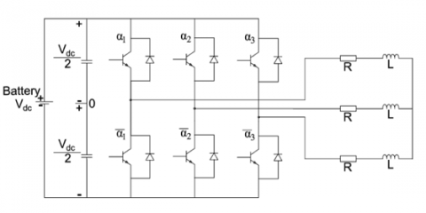
Figure 3, shows the schematic of a three-phases inverter connecting to its load, in which $\alpha_{1}, \alpha_{2},$ and $\alpha_{3}$ refer to the switch states of the phases a, b and c. We consider that the motor is star coupled.
If ($\alpha_{1,2,3}$=1), we obtain ($\overline{\alpha_{1,2,3}}$=0).
Figure 3. Brushless Direct Current Motor inverter scheme
The expression of the reference voltages at the terminals of each stator phases of the motor and the common neutral point is expressed in Eq. (13), in which $V_{a n}, V_{b n}, V_{c n}$ are the stator phase voltages between the neutral point while the connection is star coupling, and the end of the phase winding. $V_{d c}$ is the inverter supply by a battery.
$\left\{\begin{array}{l}\left(\begin{array}{l}V_{a n} \\ V_{b n} \\ V_{c n}\end{array}\right)=\frac{V_{d c}}{3} A\left(\begin{array}{c}\alpha_{1} \\ \alpha_{2} \\ \alpha_{3}\end{array}\right) \\ A=\left(\begin{array}{ccc}2 & -1 & -1 \\ -1 & 2 & -1 \\ -1 & -1 & 2\end{array}\right)\end{array}\right.$ (13)
We can model the inverter by the previous equation, having as inputs the switching signals and the Direct Current (DC) voltage supplied by the battery, and at the output the supply voltages of the three phases of the motor.
2.3.2 Inverter control
The autopilot control of the BLDCM involves being able to impose a desired current form the phases of the motor according to the rotor position. This is achieved by the full-wave offset control. Then, the output voltages are generated by commuting the arm switches to the desired voltage frequency. Each switch is controlling for 120°. There is a 60° "hole" between controlling two switches in the same sequence (disjoint control). There are six 60° electrical intervals (called sectors) of operation depending on the position of the rotor detected by the signals given by the 6-sectors sensors. In each sector, only two phases of the machine are powered, except during switching. The controls of the switches in one branch are offsetting by 120° from an adjacent branch's switches. As shown in Figure 4.
Figure 4. Full-wave offset control of BLDCM
However, since the matrix A presented in Eq. (13) is singular, the solution of the previous equation is not unique.
Then the calculation of duty cycles that involve the calculation of switch control command is not unique [31].
An additional constraint is required to solve the matrix equation. Thus, an infinity of solutions is possible to generate the duty cycles from the desired reference stator voltages. Three-phase pulse width modulation (PWM) is chosen in our case to solve that problem. In this situation, we put $V_{n o}=\frac{V_{m e d}}{2}$ where $V_{\text {med }}$, is the median voltage of the three stator reference voltages defined as follows:
If $V_{a n}<V_{b n}<V_{c n},$ then $V_{m e d}=V_{b n}$.
Hence, we obtain the Eq. (14).
$\alpha_{i}=\frac{1}{V_{d c}}\left(V_{k n}+\frac{V_{m e d}}{2}\right)+0.5 / k=a, b, c$ (14)
The control of the Brushless Direct Current Motor (BLDCM) is identical to the control of a Direct Current Motor (DCM) with separated excitation. However, we must place ourselves in Park's reference frame (d, q).
The d-axis component of the stator current plays the role of excitation and allows the value of the flux in the machine to be adjusted. The q-axis element plays the role of the armature current and controls the torque .
In order to work at maximum torque, our strategy consists in imposing quadratic current $i_{q}$ at a corresponding value, while maintaining zero the direct current $i_{d}$. The speed is regulated in cascade by imposing the desired speed value on the q-axis. As BLDCM is without salience, we obtain $L_{d}=L_{q}=\mathrm{L}$.
3.1 Current control
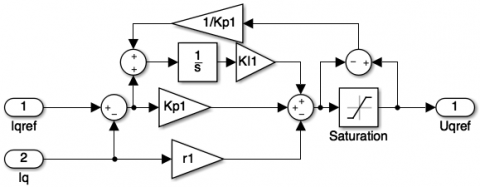
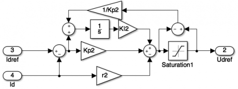
The stator currents in the Park reference frame are to be controlled by using anti-windup Proportional Integral Controllers (PI Controller), the functional schematics are shown in Figure 5 and Figure 6.
Figure 5. Anti-Windup PI Controller applied to the quadratic current $I_{q}$
Figure 6. Anti-Windup PI Controller applied to the direct current $I_{d}$
where, Kp1, Kp2, KI1, KI2, r1 and r2 shown in Figure 5 and Figure 6 are presented in Eqns. (15) and (16).
$\left\{\begin{array}{c}K p 1=2 L_{q} \omega_{c 1} \zeta_{1} \\ K I 1=L_{q} \omega_{c 1}^{2} \\ r 1=K p 1-R\end{array}\right.$ (15)
$\left\{\begin{array}{c}K p 2=2 L_{d} \omega_{c 2} \zeta_{2} \\ K I 2=L_{d} \omega_{c 2}^{2} \\ r 2=K p 2-R\end{array}\right.$ (16)
where,
$\omega_{c 1} \omega_{c 2}$ are the desired bandwidth.
$\zeta_{1}$ et $\zeta_{2}$ are the overshoot of the regulation at the quadratic current and respectively direct current.
3.2 Angular velocity control using Proportional Integral Controller (PI Controller)
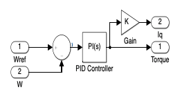
Once the regulation of the current loop is validated, it is possible to set up in cascade the desired speed (angular velocity) loop. The possibility of cascading is justifying by the fact that the electrical and mechanical time constants have a ratio greater than 10 in the majority of the electrical motor. Thus, a Proportional Integral corrector is adequate to establish the speed loop at the desired dynamic value. The block diagram of the global regulation applied to the q axis is shown in Figure 7.
Figure 7. Cascading Proportional Integral angular velocity regulation
The transfer function of the angular velocity controller is given in Eqns. (17) and (18).
$P I(s)=K p 3+\frac{K I 3}{s}$ (17)
$\left\{\begin{array}{c}K p 3=\frac{4}{3 K e}\left(2 J \omega_{c 3} \zeta_{3}-f_{v}\right) \\ K I 3=\frac{4}{3 K e} J \omega_{c 3}^{2} \\ K e=p \Phi_{m}\end{array}\right.$ (18)
The bandwidth $\omega_{c 3}$ is chosen for the speed loop at least 10 times lower than the current loop to ensure a valid cascade.
3.3 Angular velocity control using Fuzzy Logic Controller (FLC)
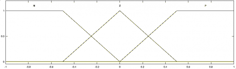
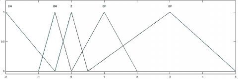
Another technique to control the angular velocity once the validation of the current regulation is done, is the Fuzzy Logic Controller (FLC). This type of controller is widely applied for solving non-linear systems problems. Hence, in this paper a Mamdani-type of FLC is adopted for controlling the inputs (the error and the error variation), and the output (the torque generated by the motor). Each input has three trapezoidal membership function (Negative (N), Zero(Z), Positive (P)), and the output has five triangular membership function (Big Negative (BN), Small Negative (SN), Zero (Z), Small Positive (SP) and Big Positive (BP)). The structures of all these memberships are shown in Figures 8, 9 and 10.
Figure 8. The membership function of the input error
Figure 9. The membership function of the input error variation
Figure 10. The membership function of the output torque
These memberships are governed by the following nine rules bases as described in Table 1.
Table 1. Fuzzy logic controller rules of inference
|
Error
Error Variation |
N |
Z |
P |
|
N |
BN |
BN |
Z |
|
Z |
BN |
Z |
SP |
|
P |
SP |
BP |
BP |
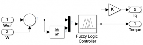
The block diagram of the global regulation applied to the q axis is shown in Figure 11.
Figure 11. Cascading Fuzzy Logic Controller for angular velocity Regulation
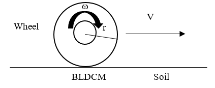
The driven wheel is defined as shown in Figure 12.
Figure 12. Driven wheel model
The linear velocity of the wheel is defined in Eq. (19).
$V=r \omega(1-s)$ (19)
where,
r is the radius of the wheel.
s is the slipping or sliding ratio.
While the wheel rotates freely, the Eq. (19) is transformed into the Eq. (20).
$V=r \omega$ (20)
By ignoring the resistive and inductive voltages across the stator windings, the power consumed by the motor is defined as shown in Eq. (21).
$P_{c}=i_{s} V_{s}$
$i_{s}=\sqrt{i_{d}^{2}+i_{q}^{2}} \leq i_{n}$
$V_{s}=\sqrt{\left(p \omega L i_{q}\right)^{2}+(p \omega)^{2}\left(\Phi_{m}+L i_{d}\right)} \leq V_{n}$ (21)
in which, $i_{n}$ is the nominal current of the motor, $V_{n}$ the nominal voltage of the motor.
Hence, the power consumed by the motor is defined as follows.
$P_{c}=\sqrt{i_{d}^{2}+i_{q}^{2}} \sqrt{\left(p \omega L i_{q}\right)^{2}+(p \omega)^{2}\left(\Phi_{m}+L i_{d}\right)}$
$\leq i_{n} V_{n}$ (22)
While regulating direct and quadratic current to work at maximum torque, we obtain $i_{d}$=0.
$P_{c}=p \omega i_{q} \sqrt{\left(L i_{q}\right)^{2}+\left(\Phi_{m}\right)^{2}} \leq i_{n} V_{n}=P_{n}$ (23)
in which, $P_{n}$ is the nominal power of the motor.
The effective power required to function the motor is defined as follows:
$P_{u}=C_{e m} \omega$ (24)
From the Eq. (12), we obtain the Eq. (25).
$P_{u}=\frac{3}{4} p i_{q} \Phi_{m} \omega$ (25)
The energetic efficiency of the motor is defined in Eq. (26) as follows.
$\eta=\frac{P_{u}}{P_{c}}=\frac{1}{2} * \frac{\frac{3}{2} \Phi_{m}}{\sqrt{\left(L i_{q}\right)^{2}+\left(\Phi_{m}\right)^{2}}}$ (26)
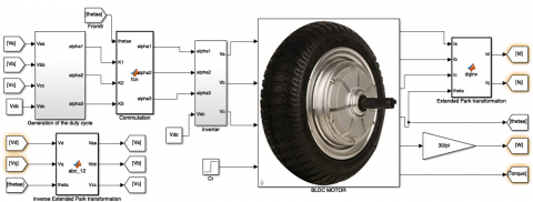
The block diagram of the BLDCM attached to its control system was modeled using the mathematical equations established previously. The system is running using the MATLAB-Simulink Library as shown in Figure 13 and Figure 14.
Figure 13. Model of BLDC in park reference frame
This allowed obtaining the angular velocity, voltage characteristics, and the behavior of the various back-electromotive forces (back-EMF), taking into account the parameters of the BLDCM as shown in the Table 2.
The results of the simulation without regulation are shown in Figure 15, Figure 16, Figure 17, Figure 18, Figure 19, Figure 20 and Figure 21.
Figure 14. Closed-Loop angular velocity control
Table 2. Characteristics of the motor
|
Nominal power (W) |
250 |
|
Dc link voltage (V) |
36 |
|
Maximum rotor-flux (Wb) |
1.255 e-2 |
|
Viscous friction coefficient (Nm$\mathrm{rad}^{-1} \mathrm{~s}^{-1}$) |
1.6e -3 |
|
Phase resistance (mW) |
500 |
|
Phase inductance (mH) |
0.68 |
|
Maximum speed (rpm) |
3000 |
|
Pairs of poles |
4 |
|
Moment of inertia (Kgm2) |
0.06 |
|
The radius of the wheel (m) |
0.20 |
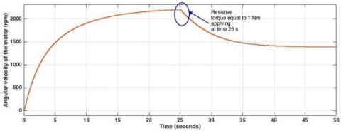
Figure 15. Angular velocity of the motor as a function of time (rpm) while rotating freely
Figure 16. The motor angular velocity while applying a resistive torque equal to 1Nm
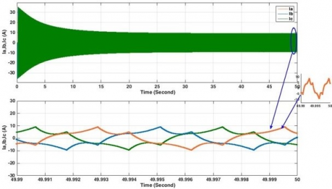
Figure 17. Current at the phases a, b and c
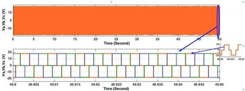
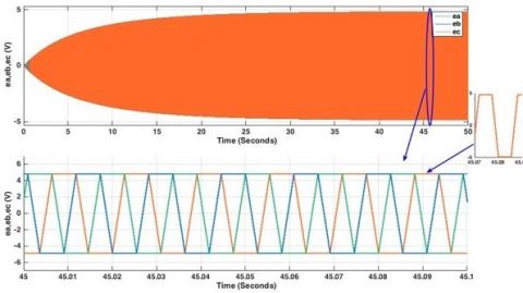
Figure 18. The voltage at the phases a, b and c
Figure 19. The back-EMF at the phases a, b and c
Figure 20. The torque generated by the motor
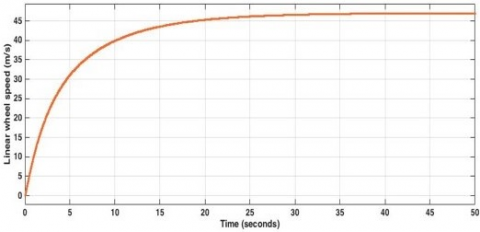
Figure 21. The linear speed of the wheel in the case of friction without slipping as a function of time
The results of the BLDCM modeling without regulation respect its trapezoidal control system.
Since the motor has a low inductance, and when the motor is functioning in an open loop, the noise due to the cutting of the inverter cannot be smoothed by the motor. Then, we obtain very noisy currents $i_{d}$ and $i_{q}$ as shown in Figure 22 and Figure 23.
The desired dynamics in closed-loop is a second-order behavior with the following characteristics: $f_{c 1}=f_{c 2}=\omega_{c 1} / 2 \pi=\omega_{c 2} / 2 \pi=2 \mathrm{KHz}$ and $\zeta_{1}=\zeta_{2}=0.1$. Thus, we obtain the following graphs as follows.
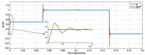
Figure 22. $i_{q}$ response during regulation of the current
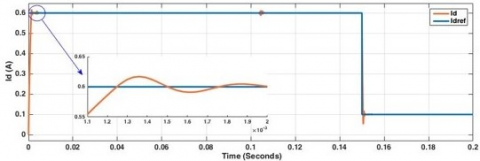
Figure 23. $i_{d}$ response during regulation of the current
Figure 24. Speed response during regulation of the speed
During the current regulation, we notice that the obtained current follows its reference. Thus, the current regulator is performant.
The cascaded speed-loop is realized using the existing current loop, keeping the same current regulators. The desired angular velocity is done using two methods: The first is Proportional Integral Controller whose dynamic loop is a 2nd order behavior with the following characteristics: $f_{c 3}=\omega_{c 3} / 2 \pi=200 \mathrm{~Hz}$ and $\zeta_{3}=0.1$, the second is using Fuzzy Logic Controller.
Hence, we obtain the following graphs as presented in Figure 24, Figure 25, Figure 26, Figure 27 and Figure 28.
Figure 25. $i_{q}$ response during regulation of the speed
Figure 26. $i_{d}$ response during regulation of the speed
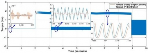
Figure 27. Torque generated during regulation of the angular velocity
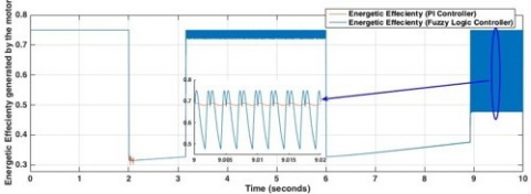
Figure 28. Energetic efficiency of the motor during regulation of the speed
We can, therefore, observe that the angular velocity follows its reference by using both; the Proportional Integral Controller (PI Controller) and the Fuzzy Logic Controller (FLC). However, while we apply the PI Controller, we notice a very slight overshoot (2nd order behavior), and for the FLC, the regulation is done without overshoot. Also, the time response for the PI Controller is less than the FLC. Thus, we notice that the PI Controller is more performing than the FLC despite the overshoot. The torque ripples are reduced in the case of FLC compared to the PI Controller when we achieve the steady state. Also, the Power ripples are reduced in the case of PI Controller compared to the FLC. Thus, we get a good performance in closed-loop speed while using PI Controller. The current loop (inner loop) is always performing although it generates a noise caused by the inverter. Thus, the current $i_{d}$ is to be zero and the current $i_{q}$ follows its reference generated by the angular velocity controller. In This case, the power efficiency of the motor exceeds 70% of the power consumed by the motor while the friction is not applied. Thus, the further work will be the optimization of the energy while the wheel moves over deformable soil.
In this paper, we presented the Brushless Direct Current Motor (BLDCM) with Trapezoidal back-Electromotive Force (back-EMF) and its mathematical model, as well as the control of this kind of machine, using the extended park transformation in order to regulate the direct and quadratic current to control the motor angular velocity with the help of two types of controllers; the Proportional Integral Controller (PI controller) and the Fuzzy Logic Controller (FLC), to finally control the torque, This torque generated by the motor must be both maximizing in value and minimizing in ripples. giving at the end the energetic efficiency of the motor while the wheel is rotating freely. The results of all these assumptions are validated using MATLAB Simulink Software to compare the two modes of controllers in terms of performance and efficacity.
Optimizing the consumed energy while controlling the velocity of the driven wheel of the robot navigating a deformable soil (while sliding), will be the subject of further works.
The authors of this paper are thankful to the Ministry of Higher Education and Scientific Research of Morocco (MESRSFC), and the National Center for Scientific and Technical Research of Morocco (CNRST) for financing this project.
|
BLDCM |
Brushless direct current motor |
|
DCM |
Direct current motor |
|
back-EMF |
Back-electromotive force |
|
PWM |
Pulse Width Modulation |
|
FOC |
field-oriented control |
|
PID Controller |
Proportional Integral Derivative Controller |
|
PI Controller |
Proportional Integral Controller |
|
FLC |
Fuzzy Logic Controller |
|
R |
Phase resistance of the motor, W |
|
L |
Phase inductance of the motor, H |
|
$L_{d}, L_{q}$ |
direct inductance and quadratic inductance, H |
|
EMF |
Electromotive force of the motor, V |
|
P ($\Theta_{e}$) |
passage matrix |
|
$V_{a}, V_{b}, V_{c}$ |
Voltage between end of phase winding and the middle of the DC voltage source, V |
|
$V_{a n}, V_{b n}, V_{c n}$ |
The stator phase voltage between a neutral point in the star connection and the end of the phase winding, V |
|
$V_{d}, V_{q}$ |
The voltage at park transformation, V |
|
$i_{a}, i_{b}, i_{c}$ |
The stator phase currents, A |
|
$i_{d}, i_{q}$ |
The currents at park transformation, A |
|
$\mathrm{e}_{a}, \mathrm{e}_{b}, \mathrm{e}_{c}$ |
The back electromotive force at phases, V |
|
$\Phi_{m}$ |
The maximum flux produced at the stator, Wb |
|
p |
The number of pole pairs |
|
tra |
Trapezoidal function |
|
J |
the inertia of the rotor, Kgm2 |
|
$C_{e m}$ |
the motor torques, Nm |
|
$C_{r}$ |
The resistance torques, Nm |
|
$f_{v}$ |
The viscous friction coefficient Nm$\operatorname{rad}^{-1} s^{-1}$ |
|
k |
The compensation of the variable after park transformation |
|
r |
Wheel radius, m |
|
s |
Slipping ratio |
|
$V_{d c}$ |
The inverter supply by a battery, V. |
|
Greek symbols |
|
|
a |
The axis in Clark transformation |
|
b |
The axis in Clark transformation |
|
$\Theta$ |
The mechanical position of the rotor, rad |
|
$\Theta_{e}$ |
The electrical position of the rotor, rad |
|
µ |
The compensation of the variable after park transformation |
|
$\omega$ |
Angular velocity of the motor, rad-1 |
|
$\omega_{c 1} \omega_{c 2}$ |
The desired bandwidth while current regulation, rad-1 |
|
$\omega_{c 3}$ |
The desired bandwidth while speed regulation, rad-1 |
|
$\zeta_{1}$ et $\zeta_{2}$ |
The overshoot of the current regulation |
|
$\zeta_{3}$ |
The overshoot of the speed regulation |
|
$\eta$ |
Energetic efficiency |
|
$\alpha_{i}$ |
Switch state at the phase i |
[1] Gao, X.Y., Li, J.H., Fan, L.F., Zhou, Q., Yin, K.M., Wang, J.X., Song, C., Huang, L., Wang, Z.Y. (2018). Review of wheeled mobile robots’ navigation problems and application prospects in agriculture. In IEEE Access, 6: 49248-49268. https://doi.org/10.1109/ACCESS.2018.2868848
[2] Salama, S., Hajjaj, H., Salleh, K., Sahari, M. (2014). Review of research in the area of agriculture mobile robots. Lecture Notes in Electrical Engineering, 291: 107-117. https://doi.org/10.1007/978-981-4585-42-2
[3] Tushar, Q., Bhuiyan, M., Sandanayake, M., Zhang, G.M. (2019). Optimizing the energy consumption in a residential building at different climate zones: Towards sustainable decision making. Journal of Cleaner Production, 233: 634-649. https://doi.org/10.1016/j.jclepro.2019.06.093
[4] Zhang, Q., Reid, J.F., Noguchi, N. (1999). Agricultural vehicle navigation using multiple guidance sensors. Proc. Int. Conf. F. Serv. Robot., pp. 293-298.
[5] Gamazo-Real, J.C., Vázquez-Sánchez, E., Gómez-Gil, J. (2010). Position and speed control of brushless dc motors using sensorless techniques and application trends. Sensors, 10(7): 6901-6947. https://doi.org/10.3390/s100706901
[6] Gabriel, D.L., Meyer, J., Du Plessis, F. (2011). Brushless DC motor characterisation and selection for a fixed wing UAV. IEEE AFRICON Conf., pp. 13-15. https://doi.org/10.1109/AFRCON.2011.6072087
[7] Rahman, K.M., Hiti, S. (2005). Identification of machine parameters of a synchronous motor. IEEE Trans. Ind. Appl., 41(2): 557-565. https://doi.org/10.1109/TIA.2005.844379
[8] Mamatov, A., Lovlin, S., Vaimann, T., Rassõlkin, A., Vakulenko, S., Abramian, A. (2019). Modified technique of parameter identification of a permanent magnet synchronous motor with PWM inverter in the presence of dead-time effect and measurement noise. Electron., 8(10): 1200. https://doi.org/10.3390/electronics8101200
[9] Demić, M. (1997). Identification of vibration parameters for motor vehicles. Veh. Syst. Dyn., 27(2): 65-88. https://doi.org/10.1080/00423119708969323
[10] Karaliunas, B. (2011). Study on the characteristics of electronically commutated motor. Elektron. Ir Elektrotechnika, 109(3): 31-34. https://doi.org/10.5755/j01.eee.109.3.165
[11] Poovizhi, M., Kumaran, S.M., Ragul, P., Priyadarshini, L.I., Logambal, R. (2017). Investigation of mathematical modelling of brushless dc motor(BLDC) drives by using MATLAB-SIMULINK. 2017 International Conference on Power and Embedded Drive Control (ICPEDC), Chennai, pp. 178-183. https://doi.org/10.1109/ICPEDC.2017.8081083
[12] Lee, K.M., Zhou, D. (2004). A real-time optical sensor for simultaneous measurement of three-DOF motions. IEEE/ASME Trans. Mechatronics, 9(3): 499-507. https://doi.org/10.1109/TMECH.2004.834642
[13] Jeddi, N., El Amraoui, L., Tadeo, F. (2016). Modelling and simulation of a BLDC motor speed control system for electric vehicles. Int. J. Electr. Hybrid Veh., 8(2): 178-194. https://doi.org/10.1504/IJEHV.2016.078369
[14] Rai, T., Debre, P. (2016). Generalized modeling model of three phase induction motor. 2016 Int. Conf. Energy Effic. Technol. Sustain. ICEETS 2016, pp. 927-931. https://doi.org/10.1109/ICEETS.2016.7583881
[15] Qu, J., Teeple, C.B., Oldham, K.R. (2017). Modeling legged microrobot locomotion based on contact dynamics and vibration in multiple modes and axes. J. Vib. Acoust. Trans. ASME, 139(3): 031013. https://doi.org/10.1115/1.4035959
[16] Jiang, W., Huang, H., Wang, J., Gao, Y., Wang, L. (2017). Commutation analysis of brushless DC motor and reducing commutation torque ripple in the two-phase stationary frame. IEEE Trans. Power Electron., 32(6): 4675-4682. https://doi.org/10.1109/TPEL.2016.2604422
[17] Institute of Electrical and Electronics Engineers, ICCAR 2019 : 2019 5th International Conference on Control, Automation and Robotics : proceedings : April 19-22, 2019, Beijing, China.
[18] Rao, C.N.N., Sukumar, G. (2018). Design and analysis of torque ripple reduction in Brushless DC motor using SPWM and SVPWM with PI control. Eur. J. Electr. Eng., 20(1): 7-22. https://doi.org/10.3166/EJEE.20.7-22
[19] Wang, F., Zhang, Z., Mei, X., Rodríguez, J., Kennel, R. (2018). Advanced control strategies of induction machine: Field oriented control, direct torque control and model predictive control. Energies, 11(1): 120. https://doi.org/10.3390/en11010120
[20] Habibullah, M., Lu, D.D.C., Xiao, D., Rahman, M.F. (2016). A simplified finite-state predictive direct torque control for induction motor drive. IEEE Trans. Ind. Electron., 63(6): 3964-3975. https://doi.org/10.1109/TIE.2016.2519327
[21] Nikzad, M.R., Asaei, B., Ahmadi, S.O. (2018). Discrete Duty-Cycle-Control method for direct torque control of induction motor drives with model predictive solution. IEEE Trans. Power Electron., 33(3): 2317-2329. https://doi.org/10.1109/TPEL.2017.2690304
[22] Zhang, Y., Xia, B., Yang, H. (2017). Performance evaluation of an improved model predictive control with field oriented control as a benchmark. IET Electr. Power Appl., 11(5): 677-687. https://doi.org/10.1049/iet-epa.2015.0614
[23] Wang, F., Wang, J., Kennel, R.M., Rodríguez, J. (2019). Fast speed control of AC machines without the proportional-integral controller: Using an extended high-gain state observer. IEEE Trans. Power Electron., 34(9): 9006-9015. https://doi.org/10.1109/TPEL.2018.2889862
[24] Ubare, P., Ingole, D., Sonawane, D. (2019). Energy-efficient nonlinear model predictive control of BLDC motor in electric vehicles. 2019 6th Indian Control Conf. ICC 2019 - Proc., pp. 194-199. https://doi.org/10.1109/ICC47138.2019.9123204
[25] Sharma, R., Gaur, P., Mittal, A.P. (2017). Optimum design of fractional-order hybrid fuzzy logic controller for a robotic manipulator. Arab. J. Sci. Eng., 42(2): 739-750. https://doi.org/10.1007/s13369-016-2306-0
[26] Gujjar, M.N., Kumar, P. (2017). Performance analysis of space vector pulse width modulation based sensor less field oriented control of brushless DC motor. Ijireeice, 5(2): 60-65. https://doi.org/10.17148/ijireeice/ncaee.2017.14
[27] Patel, J.M., Hirvaniya, H.V., Rathod, M. (2014). Simulation and analysis of brushless DC motor based on sinusoidal PWM control. International Journal of Innovative Research in Electrical, Electronics, Instrumentation And Control Engineering, 2(3): 1236-1238.
[28] Singh, J., Singh, M. (2016). Comparison and analysis of different techniques for speed control of brushless DC motor using matlab simulink. Int. J. Eng. Trends Technol., 38(7): 373-379. https://doi.org/10.14445/22315381/ijett-v38p267
[29] Majdoubi, R., Masmoudi, L., Bakhti, M., Elharif, A., Jabri, B. (2020). Parameters estimation of bldc motor based on physical approach and weighted recursive least square algorithm. Int. J. Electr. Comput. Eng., 11(1): 133-145. https://doi.org/10.11591/ijece.v11i1.pp133-145
[30] Giménez, R.B. (1995). High Performance Sensorless Vector Control of Induction Motor Drives. p. 269.
[31] Kerid, R., Bourouina, H., Yahiaoui, R. (2018). Parameter identification of PMSM using EKF with temperature variation tracking in automotive applications. Period. Eng. Nat. Sci., 6(2): 109-119. https://doi.org/10.21533/pen.v6i2.168
[32] Chandrasekaran, G., Kumarasamy, V., Chinraj, G. (2019). Test scheduling of core based system-on-chip using modified ant colony optimization. J. Eur. des Syst. Autom., 52(6): 599-605. https://doi.org/10.18280/jesa.520607