Liang Li* | Renhao Zhao | Chunlei Li
© 2020 IIETA. This article is published by IIETA and is licensed under the CC BY 4.0 license (http://creativecommons.org/licenses/by/4.0/).
OPEN ACCESS
Non-holonomic path planning is to solve the two point boundary value problem under constraints. Since it is offline and open-loop, the path planning cannot compensate for the disturbances and eliminate the errors. To solve the problems, this paper puts forward an iterative learning control algorithm that adjusts the control parameters of the path planner online through the multiple iterative computations of the target configuration error equation, under the initial configuration error and model error, and thus enhancing the accuracy of non-holonomic system path planning. Then, a simulation experiment on path planning was carried out for a chainable three-joint, non-holonomic manipulator. The results show that the iterative learning controller can eliminate the interference of initial configuration error and model error, such that each joint can move to the target configuration.
non-holonomic system, iterative learning, path planning, initial configuration error, model error
The actual control of non-holonomic system suffers from various disturbances, due to the error in the fabrication and assembly of non-holonomic machines, the insufficient resolution of the transmission system, and the uncertain accuracy of the measuring instrument [1, 2]. As a result, the actual result of motion control often deviates from the theoretical simulation value, that is, the final configuration of the system does not coincide with the target configuration [3]. The most direct solution is to plan the path again for the system to move from the actual configuration to the target configuration [4-6]. However, the secondary path planning may not yield a feasible path, not to mention achieving the desired result, under the strong nonlinearity of the mathematical models for some non-holonomic systems [7, 8].
The iterative learning control is a possible way to improve the secondary path planning. By this method, the current control input is corrected repeatedly based on the error between the previous control output and the theoretical control output, i.e. the current control input is learned from the previous control output of the system, such that the error of system control output can converge to the pre-set value [9]. Compared with state feedback [10], variable structure [11, 12] and adaptive methods [13, 14], the iterative learning control algorithm enjoys certain advantages in the motion control of nonlinear system with uncertainties, thanks to its independence from the mathematical model of the system and fast convergence speed. Considering the initial configuration error, this paper attempts to improve the motion control accuracy by designing an iterative learning controller suitable for chainable non-holonomic system, according to the iterative root-finding of nonlinear equations.
The trajectory of chainable non-holonomic system can be obtained through inverse transformation of the path of the chain variable. Let θe(t) and ze be the trajectory of the joint with initial configuration error and the corresponding chain variable, respectively. Then, the error of the joint trajectory θe(t) can be mapped as ze. Thus, the control of the error from the target configuration is equivalent to compensating the error-containing chain variable ze in the chain space. The mathematical model of the n+1 dimensional single-chain system can be expressed as [15]:
$\left\{ \begin{align} & {{{\dot{z}}}_{1}}(t)={{v}_{1}}(t) \\ & \dot{z}(t)=A(t)\cdot z(t)+B\cdot {{v}_{2}}(t) \\\end{align} \right.$ (1)
where, $A(t)=\left[\begin{array}{ccccc}
0 & 0 & \cdots & 0 & 0 \\
v_{1}(t) & 0 & \cdots & 0 & 0 \\
0 & v_{1}(t) & \cdots & 0 & 0 \\
\vdots & \vdots & \cdots & \vdots & \vdots \\
0 & 0 & \cdots & v_{1}(t) & 0
\end{array}\right]\left(A(t) \in R^{n} \times R^{n}\right)$ $B=\left[\begin{array}{l}
1 \\
0 \\
0 \\
\vdots \\
0
\end{array}\right]\left(B \in R^{n}\right) ; z(t)=\left[z_{2}(t), z_{2}(t), \cdots, z_{n+1}(t)\right]^{T}$ is the chain variable at time t ( $t \in[0, T]$ ). The initial and target configurations of z(t) can be denoted as $z^{0} \in R^{n} \text { and } z^{f} \in R^{n}$, respectively. If A(t)=A is a constant matrix, i.e. the control input v1(t) is constant, then Eq. (1) is a first-order linear time-invariant system. According to the time polynomial control law [4], the following can be derived from Eq. (1):
$v(t)=v(t,{{b}_{0}},c)$ (2)
where, $v\left(t, b_{0}, C\right)=\left[v_{1}(t), v_{2}(t)\right]^{T} \quad, \quad b_{0} \in R$; $c=\left[c_{0}, c_{1} \cdots c_{n-1}\right]$ is the control parameter vector with the same number of dimensions as the chain variable z(t). Let $\lambda_{i}(t):[0, T] \rightarrow R^{m-1}$ be an input mapping, with m being the number of dimensions (m=2 for single-chain system) and $i \in\{0,2, \cdots, n-1\}$ being linearly independent. Then, the input basis function in the linear space of the time constant input control function can be constructed as:
$\left\{ \begin{align} & {{v}_{1}}(t)={{b}_{0}} \\ & {{v}_{2}}(t)=\sum\limits_{i=0}^{n-1}{{{c}_{i}}{{\lambda }_{i}}(t)} \\\end{align} \right.$ (3)
Then, the path planning of chain system is equivalent to choosing a proper v(t), such that the chain system can move from z0 to point zf in the chained-form space within the specified time. Solving Eq. (1), we have:
$\begin{align} & {{z}^{f}}={{e}^{A(T)}}{{z}^{0}}+\int_{0}^{T}{{{e}^{A(T-t)}}B}\cdot {{v}_{2}}(t)dt \\ & ={{e}^{A(T)}}{{z}^{0}}+\sum\limits_{i=0}^{n\text{-}1}{{{c}_{i}}}\int_{0}^{T}{{{e}^{A(T-t)}}B}\cdot {{\lambda }_{i}}(t)dt \\ & =P{{z}^{0}}+Qc \end{align}$ (4)
where, P=eA(T) and $Q=\int_{0}^{T} e^{A(T-t)} B \cdot \lambda(t) d t$ are both $R^{n} \times R^{n}$ constant matrices; $\lambda(t)=\left[\lambda_{0}(t), \lambda_{1}(t), \cdots, \lambda_{n-1}(t)\right]^{T}$ is the basis function vector. Eq. (4) shows that the state zf of the chain system at time T can be derived from the given initial condition z0 and a corresponding set of parameter vectors c.
It is assumed that the configuration variable of a chainable non-holonomic system has an initial error. This initial configuration error is denoted as $z_{e}^{0}$ after being mapped to the chain space. Under the error $z_{e}^{0}$ , the target configuration of the system can be expressed as a function of the parameter vector c. Let $z_{e}^{f}\left(c^{[k]}\right)$ be the target configuration after k iterations. Then, the linear invariant homogeneous equation with respect to parameter vector c at time T can be expressed as:
$e({{c}^{[k]}})={{z}^{f}}-z_{e}^{f}({{c}^{[k]}})\approx 0$ (5)
where, c[k] is the parameter vector after k iterations; e(c[k]) is the target configuration error function of the chain variable. Then, the iterative expressions for the control parameter vector and the velocity input can be defined as:
$c_{{}}^{^{[k]}}=c_{{}}^{^{[k-1]}}+F\cdot e(c_{{}}^{^{[k-1]}})$ (6)
${{v}^{[k]}}(t)=\sum\limits_{i=0}^{n\text{-}1}{{{c}_{i}}^{[k]}{{\lambda }_{i}}(t)}$ (7)
where, matrix $F \in R^{n} \times R^{n}$. To ensure the iterative convergence of Eq. (5), the general method is to judge the convergence features by the eigenvalues of the iterative matrix. In many cases, however, it is difficult and even impossible to solve the eigenvalues of the iterative matrix. Hence, the range of eigenvalues is estimated in engineering practices, rather than determine the exact eigenvalues. The Gershgorin circle theorem [16] is often adopted to prove that all the eigenvalues of the iterative matrix fall within the open set of the unit circle on the complex plane.
Lemma 1 (Iterative convergence) For the update Eq. (6) for the control parameter vector of the time polynomial control input, there exists an iterative matrix I-QF whose eigenvalues are located in the open unit Gershgorin disc of the complex plane, such that the target configuration error function e(c[k]) of the chain variable converges exponentially to zero.
Proof: Substituting Eq. (4) into Eq. (5), we have
$e({{c}^{[k+1]}})-e({{c}^{[k]}})=-z({{c}^{[k+1]}})+z({{c}^{[k]}})=-Q({{c}^{[k+1]}}-{{c}^{[k]}})$ (8)
Sorting equation (6) into $c^{[k+1]}-c^{[k]}=F \cdot e\left(c^{[k+1]}\right)$ and substituting it into the above equation, we have:
$e({{c}^{[k+1]}})=e({{c}^{[k]}})-QF\cdot e({{c}^{[k]}})=(I-QF)\cdot e({{c}^{[k]}})$ (9)
The controllability of the chain system (1) guarantees that, the parameter vector in Eq. (4) has a unique set of solutions under the time polynomial input and the known initial and target configurations z0 and zf. Thus, matrix Q is not singular. Let F=ηQ-, with $\eta \in R$. According to the Gershgorin circle theorem, the eigenvalues of the iterative matrix I-QF of Eq. (8) at $\eta \in(0,2)$ can be estimated as:
$D=\left\{ \lambda \left| \left| \lambda -{{a}_{ii}} \right| \right.\le 0,\lambda \in C \right\}$ (10)
where, aii is the main diagonal element of the iterative matrix I-QF and aii≡η. Therefore, the eigenvalues λ of the iterative matrix fall within the unit circle in the complex plane, indicating that Eq. (5) can converge to zero at any speed.
Q.E.D.
Since the mathematical structure of the chain system (1) guarantees the linearity of Eq. (5) is linear, Eq. (1) can also be expressed as:
$\dot{z}(t)=A(t)\cdot z(t)+B\cdot v(t)$ (11)
where, $A(t)=\left[\begin{array}{cccccc}
0 & 0 & 0 & \cdots & 0 & 0 \\
0 & 0 & 0 & \cdots & 0 & 0 \\
v_{1}(t) & 0 & 0 & \cdots & 0 & 0 \\
0 & v_{1}(t) & 0 & \cdots & 0 & 0 \\
\vdots & \vdots & \vdots & \cdots & \vdots & \vdots \\
0 & 0 & 0 & \cdots & v_{1}(t) & 0
\end{array}\right]$ ( $\mathrm{A}(t) \in R^{n+1} \times R^{n+1}$); $B=\left[\begin{array}{cc}
1 & 0 \\
0 & 1 \\
0 & 0 \\
0 & 0 \\
\vdots & \vdots \\
0 & 0
\end{array}\right] \quad\left(B \in R^{n+1} \times R^{2}\right)$; $z(t)=\left[z_{1}(t), z_{2}(t), \cdots, z_{n+1}(t)\right]^{T} \quad\left(\quad z(t) \in R^{n+1}\right)$; $v(t)=\left[v_{1}(t), v_{2}(t)\right]^{T}$.
The Eq. (5) thus constructed is a set of nonlinear fixed-length homogeneous equations with respect to the parameter vector c. This equation can be solved iteratively by the root-finding method for nonlinear equations, and its convergence can still be evaluated by Lemma 1.
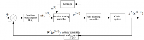
Taking a chainable three-joint non-holonomic manipulator as the object [17], the iterative learning controller was applied to the path planning with initial configuration error. The control parameter vector c was adjusted through the iterative calculation of the target configuration error function, such that the actual configuration θa of the three-joint manipulator can converge to the expected value at time T, despite the initial configuration error. Figure 1 illustrates the iterative learning control system.
Figure 1. Block diagram of our iterative learning control system
The iterative learning control algorithm can be implemented in the following steps:
Step 1. According to the polynomial path planner, calculate the theoretical value zf and the chain variable under initial configuration error $z_{e}^{f}$ of the chain system Eq. (1), and solve the target configuration error function e(c[0]) of the chain variable.
Step 2. Solve the matrices P and Q in Eq. (4). It can be seen from Eq. (3) that the input basis function vector can be expressed as $\lambda(t)=\left[\lambda_{0}(t), \lambda_{1}(t), \lambda_{2}(t)\right]^{T}=\left[1, t, t^{2}\right]^{T} \quad(t \in[0, T])$. According to Eq. (4), there exists an exponential mapping $\Phi_{e}: A(T) \rightarrow P \in R^{3 \times 3}$. Then, P=eA(T) can be expanded as:
$P=I+A(T)T+\frac{A{{(T)}^{2}}}{2!}{{T}^{2}}+\frac{A{{(T)}^{3}}}{3!}{{T}^{3}}+\cdots =\left[ \begin{matrix} 1 & 0 & 0 \\ {{b}_{0}}T & 1 & 0 \\ {{({{b}_{0}}T)}^{2}}/2 & {{b}_{0}}T & 1 \\\end{matrix} \right]$ (12)
where, $A(T)=\left[\begin{array}{ccc}
0 & 0 & 0 \\
b_{0} & 0 & 0 \\
0 & b_{0} & 0
\end{array}\right]$. The following can be derived from Eq. (4):
$\begin{align} & Q=\int_{0}^{T}{\left[ \begin{matrix} 1 & 0 & 0 \\ {{b}_{0}}(T-t) & 1 & 0 \\ {{b}_{0}}^{2}{{(T-t)}^{2}}/2 & {{b}_{0}}(T-t) & 1 \\\end{matrix} \right]\cdot \left[ \begin{matrix} 1 \\ 0 \\ 0 \\\end{matrix} \right]\cdot [\begin{matrix} 1 & t & {{t}^{2}} \\\end{matrix}]}dt \\ & =\left[ \begin{matrix} T & {{T}^{2}}/2 & {{T}^{3}}/3 \\ {{b}_{0}}{{T}^{2}}/2 & {{b}_{0}}{{T}^{3}}/6 & {{b}_{0}}{{T}^{4}}/12 \\ {{b}_{0}}^{2}{{T}^{3}}/6 & {{b}_{0}}^{2}{{T}^{4}}/24 & {{b}_{0}}^{2}{{T}^{5}}/60 \\\end{matrix} \right]\end{align}$ (13)
Step 3. Establish the termination condition of the iteration. According to the configuration error of the chain variable after k iterations, the norm of the target configuration error function can be defined as:
$pe=\left\| e(c_{{}}^{^{[k]}}) \right\|=\left\| {{z}^{f}}-z_{e}^{f}({{c}^{[k]}}) \right\|$ (14)
The iteration should be terminated when pe≤δ, where $\delta \in R^{+}$ is a sufficiently small given positive value.
Step 4. Substitute the condition F=ηQ- of Lemma 1 into the iterative calculation of Eq. (6), and iteratively update the parameter vector c[i] according to Step 3 until the target configuration error function in Eq. (5) satisfies the termination condition. Then, the value of c[k+1] can be obtained as:
$c_{{}}^{^{[k+1]}}=c_{{}}^{^{[k]}}+\eta {{Q}^{-}}\cdot e(c_{{}}^{^{[k]}})$ (15)
Step 5. Substitute c[k+1] into the expression of zi(t), and solve the iteratively corrected trajectory via inverse transformation. If F=ηQ- in Eq. (6) equals the negative of the Jacobian inverse matrix of parameter vector c in Eq. (5) at η=1, we have:
$\eta {{Q}^{-}}=-Jab{{(c)}^{-}}$ (16)
Obviously, the iterative error correction algorithm in Eq. (6) for the parameter vector c is a Newton’s iteration method. The geometric meaning is: the linear operator described by Jab(c) optimizes the approximation of c[k] to c[k+1].
The chain equations and input equations of three-joint non-holonomic manipulator can be obtained as follows through coordinate transformation of the kinematics equation of the manipulator (the mechanical form, kinematics equation and coordinate transformation method are described in Reference [17]):
$\left\{ \begin{align} & {{z}_{4}}={{\theta }_{3}} \\ & {{z}_{3}}=\frac{\partial {{z}_{4}}}{\partial \underline{{{q}_{4}}}}\underline{{{f}_{4}}}(\underline{{{q}_{3}}})=(\frac{{{k}_{3}}}{{{k}_{g}}}){{\cos }^{3}}{{\theta }_{2}} \\ & {{z}_{2}}=\frac{\partial {{z}_{3}}}{\partial \underline{{{q}_{3}}}}\underline{{{f}_{3}}}(\underline{{{q}_{2}}})=\frac{-3{{k}_{3}}{{k}_{2}}}{k_{g}^{2}}{{\cos }^{2}}\theta _{1}^{{}}{{\cos }^{2}}\theta _{2}^{{}}\sin {{\theta }_{2}} \\ & {{z}_{1}}={{\phi }_{2}} \\\end{align} \right.$ (17)
$\left\{ \begin{array}{*{35}{l}} {{v}_{1}}={{u}_{1}}={{\phi }_{2}} \\ {{v}_{2}}=\frac{3k_{2}^{2}{{k}_{3}}}{k_{g}^{3}}c_{1}^{4}(2{{c}_{2}}s_{2}^{2}-c_{2}^{3}){{u}_{1}}+\frac{6{{k}_{2}}{{k}_{3}}}{k_{g}^{2}}{{c}_{1}}{{s}_{1}}c_{2}^{2}{{s}_{2}}{{u}_{2}} \\\end{array} \right.$ (18)
where, k2, k3 and k3 are the structural size coefficients of the manipulator; θ=[θ1 θ2 θ3)]T and [u1 u2]T are the joint space and input space of the manipulator, respectively.
For the three-joint non-holonomic manipulator, the path planning based on iterative learning control is to determine the angular velocity inputs u1 and u2 of the servo motor, such that all the joints can move from the error-containing initial configuration $\theta_{e}^{0}$ accurately to the target configuration θf, under the joint action of the polynomial control law (2) and iterative update parameter vector c[k+1]. Unlike the path planning of manipulator under holonomic constraint, the path planning of each joint of non-holonomic manipulator must satisfy the non-holonomic constraint, instead of being random.
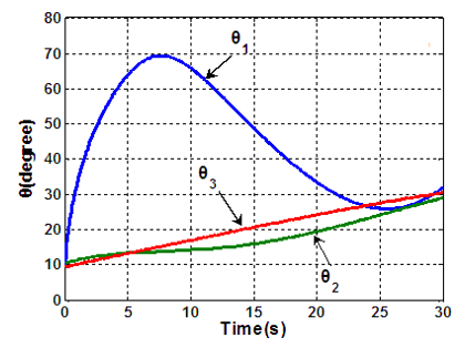
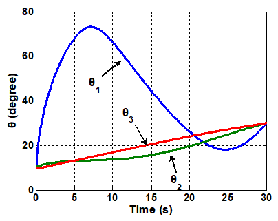
Let $\theta_{e}^{0}$=[9°, 11°, 9°]T, θ0=[10°, 10°, 10°]T and θf=[30°, 30°, 30°]T be the error-containing initial configuration, the theoretical initial configuration and the target configuration, respectively. Then, the initial configuration error is 1°. Under these configurations, the path planning of three-joint manipulator was simulated with and without initial configuration errors and the results were recorded in Figures 2 and 3 below. The results show that the small initial configuration error (1°) has a great impact on the path planning result of the system, twisting the geometric shape of the path and preventing the joints from reaching the target configuration in the specified time.
Figure 2. Angular displacement trajectories of the joints in the simulation without initial configuration error
Figure 3. Angular displacement trajectories of the joints in the simulation with initial configuration error of 1°
Then, the iterative learning algorithm was applied to the simulation with initial configuration error of 1°. The simulation results after four iterations are displayed in Figures 4 and 5 below. It can be seen that the three-joint non-holonomic manipulator moved from the error-containing initial configuration θ0=[9°, 11°, 9°]T to the target configuration θf=[30°, 30°, 30°]T after a period of time. The position error $p e$ of the chain variable changed with the number of iterations, in that the target configuration error function e(c[k]) of the system converged exponentially to the target configuration.
Figure 4. Iterative simulation curve with 1° error
Figure 5. Iterative convergence rate of the error (exponential convergence)
According to the evaluation index of linear approximation of non-holonomic systems [18], the iterative trajectory of the system is not satisfactory at φ2=36.6°, and the planned path of joint 1 deviated from the linear reference path (the segment between the initial and target configurations) by 59.63° at the most. There were 2 extreme values on the trajectory relative to the reference path, indicating that joint 1 turned twice during the movement.
Although the iterative learning algorithm can eliminate the error of the target configuration, the path planning result of the system is greatly affected by a small initial error (1°), as evidenced by the significant distortion of the geometric shape of the planned path. This means the system has a poor fault tolerance, which hinders the iterative linear approximation of the path. Compared with linear path, the non-holonomic path fluctuates and zigzags along the way. To solve the problem, it is necessary to identify the nonlinear mapping between the chain space and configuration space, and select the input parameters based on the error tolerance coefficient, thus reducing the sensitivity of the manipulator system to the initial error and enhancing the open-loop robustness and operability of path planning. The specific steps are detailed in Reference [18].
Under continuous disturbance, formula (1) can be rewritten as:
$\dot{z}(t)=A(t)\cdot z(t)+B\cdot v(t)+\delta (z(t),v(t),t)$ (19)
where, δ is a disturbance function that is continuously differentiable about z(t) and v(t). Solving formula (19) in interation interval i=([k], [k+1]):
$z_{e}^{f,[i]}={{e}^{AT}}z_{0}^{[i]}+\int_{0}^{T}{{{e}^{A(T-t)}}B}\cdot {{v}^{[i]}}(t)dt+\int_{0}^{T}{{{e}^{A(T-t)}}}\delta ({{z}^{[i]}}(t),{{v}^{[i]}}(t),t)dt$ (20)
where, the first two terms are the steady-state output of the undisturbed chain system; the last term is the steady-state output difference between the disturbed chain system at time T in the iteration interval ([k], [k+1]) and the undisturbed chain system. Then, the error function of the steady-state output of the system can be expressed as:
${{\tilde{\varepsilon }}^{[i]}}=\int_{0}^{T}{{{e}^{A(T-t)}}}\delta ({{z}^{[i]}}(t),{{v}^{[i]}}(t),t)dt$ (21)
Formula (21) is essentially a partial solution of formula (20). From the nature of the slution to first-order differential equation and the controllable condition of the nonholonomic system, it can be seen that formula (21) is a continuously differentiable function of the parameter vector c. Under continuous interference, the target configuration of system (19) after k iterations can be written as:
$z_{e}^{f,[i]}=P{{z}^{0}}+Q{{c}^{[k]}}+{{\varepsilon }^{[k]}}$ (22)
where, $P=e^{A(T)} ; Q=\int_{0}^{T} e^{A(T-t)} B \cdot \lambda(t) d t ; \varepsilon^{[k]}$ is the residual error between the actual target configuration and theoretical target configuration. Then, the error function of the target configuration can be expressed as:
$\begin{align} & e(c_{{}}^{^{[k]}})={{z}^{d}}-z_{e}^{^{[k]}}(T)={{z}^{d}}-(P{{z}^{0}}+Q{{c}^{[k]}}+{{\varepsilon }^{[k]}}) \\ & ={{z}^{d}}-(P{{z}^{0}}+Q(c_{{}}^{^{[k-1]}}+F\cdot e(c_{{}}^{[k-1]}))+{{\varepsilon }^{[k]}}) \end{align}$ (23)
Substituting this into formula (5):
$\begin{align} & e(c_{{}}^{^{[k]}})=e(c_{{}}^{^{[k-1]}})-QFe(c_{{}}^{^{[k-1]}})-{{\varepsilon }^{[k]}}+{{\varepsilon }^{[k-1]}} \\ & =(I-QF)e(c_{{}}^{^{[k-1]}})+({{\varepsilon }^{[k-1]}}-{{\varepsilon }^{[k]}})\end{align}$ (24)
After k iterations, the system error induced by dynamic disturbance can be expressed as:
${{\zeta }^{[k-1]}}={{\varepsilon }^{[k-1]}}-{{\varepsilon }^{[k]}}$ (25)
where, $\zeta^{[k]}$ is the bounded continuous differentiable function about parameter vector c (which guarantees boundedness). According to the Lipschitz condition, there exists a Lipschitz constant k>0 in the definition domain of c. Then, $\zeta^{[k]}$ satisfies:
$\left| {{\zeta }^{[k]}} \right|=\left| {{\varepsilon }^{[k]}}-{{\varepsilon }^{[k+1]}} \right|\le k\cdot \left| {{c}^{[k]}}-{{c}^{[k+1]}} \right|=k\cdot \left| -F\cdot e(c_{{}}^{^{[k]}}) \right|$ (26)
Let F=ηQ-. Then, formula (26) can be rewritten as:
$\left| {{\zeta }^{[k]}} \right|\le k\eta p\left| e(c_{{}}^{^{[k-1]}}) \right|$ (27)
where, $p=\left|Q^{-}\right|$. Obviously, if the consistency index perturbation term $\left|\zeta^{[k]}\right|$ induced by dynamic disturbance through iterations can converge to zero, there always exists a coefficient $\sigma \in R^{+}$ that makes $\frac{\sigma}{k \eta p} \ll 1$. Substituting this coefficient into formula (21):
$\left| {{\zeta }^{[k]}} \right|=\sigma \left| {{{\tilde{\zeta }}}^{[k]}} \right|=\sigma \left| {{{\tilde{\varepsilon }}}^{[k]}}-{{{\tilde{\varepsilon }}}^{[k+1]}} \right|$ (28)
According to formula (28), the chain system can be reconstructed to satisfy the relevant conditions:
$\dot{z}(t)=A(t)\cdot z(t)+B\cdot v(t)+\sigma \cdot \delta (z(t),v(t),t)$ (29)
where, σ is a sufficiently small positive real number that needs to satisfy $\frac{\sigma}{k \eta p} \ll 1$, such that the consistency index of formula (24) can converge to zero after the system iterates by formula (6) under dynamic disturbance.
As shown in formula (27), the perturbation term of the chain system is completely decoupled. Hence, the chain system (1) can be divided into two parts for iterative calculation. This not only improves the efficiency of iterative convergence, but also reduces the algorithm difficulty. On the contrary, chain system (11) complicates the algorithm and slows down the iterative convergence.
Suppose the two contacting discs (A1 and C1) on the rotation axis of joint 1 in three-joint non-holonomic manipulator [17] have model errors with the corresponding turntables (B1 and D1): the working radius r1e of each disc is 103% of the nominal radius; the actual distance Re from the contact point of each disc and turntable B1 to the rotation axis of that turntable is 105% of the design distance; the actual distance r3e from the contact point of each disc and turntable D1 to the rotation axis of that turntable is 107% of the design distance.
Since joint 1 is directly driven by motor, its angular displacement θ1 is not affected by the initial configuration error. The increase of radius r1e of disc A1 causes the linear velocity and displacement of the disc to increase proportionally. Whereas the manipulator has an open motion transmission chain, the model errors of the two discs will propagate along the chain, and affect the trajectories of all joints, except the angular displacement θ1 of joint 1. In addition, the initial configuration error will induce time-variation in the control input of the chain system, according to the input feedback transformation formula of chain transformation.
Except for model error, the parameters are consistent with those in Li’s work [17]. The simulation results show that the actual target configuration $\theta_{a}^{f}=\left[30^{\circ}, 28^{\circ}, 28^{\circ}\right]^{T}$ of the three-joint manipulator at the end of movement deviated from the specified target configuration, owing to the presence of model error (Figure 6).
Figure 6. The simulation curves under model error (φ2=32.8°, da=22.84°, tp=1)
Through iterative learning, the coefficients in formula (27) can be expressed as:
$\eta \in (0,2)$ (30)
$k=\left| Jab({{\varepsilon }^{[k]}}(c)) \right|=\left| \begin{matrix} t & {{t}^{2}}/2 & {{t}^{3}}/3 \\ b_{0}^{[i]}{{t}^{2}}/2 & b_{0}^{[i]}{{t}^{3}}/6 & b_{0}^{[i]}{{t}^{4}}/12 \\ b{{_{0}^{[i]}}^{2}}{{t}^{3}}/6 & b{{_{0}^{[i]}}^{2}}{{t}^{4}}/24 & b{{_{0}^{[i]}}^{2}}{{t}^{5}}/60 \\\end{matrix} \right|$ (31)
$p=\left| {{Q}^{-}} \right|=\left| \begin{matrix} 3/T & -24/(b_{0}^{[i]}{{T}^{2}}) & 60/(b{{_{0}^{[i]}}^{2}}{{T}^{3}}) \\ -24/{{T}^{2}} & 168/(b_{0}^{[i]}{{T}^{3}}) & 360/(b{{_{0}^{[i]}}^{2}}{{T}^{4}}) \\ 30/{{T}^{3}} & -180/(b_{0}^{[i]}{{T}^{4}}) & 360/(b{{_{0}^{[i]}}^{2}}{{T}^{5}}) \\\end{matrix} \right|$ (32)
Figure 7. The iterative simulation curves under model error (φ2=32.8°, da=28.05°, tp=1)
Figure 8. The iterative convergence speed of model error (exponential convergence)
Figure 7 presents the simulation results at t=T and kηp=η. Figure 8 is the iteratively convergence speed. After four iterations, the non-holonomic manipulator can converge near the target configuration θf, under the conditions of formula (14).
Based on the root-finding method for nonlinear equations, this paper proposes an iterative learning control algorithm, and proves through mathematical deduction that the controller can make the chain system converge to the target value at any speed with the initial configuration error and model error. Then, the author carried out a simulation experiment on path planning for a chainable three-joint manipulator. The results show that the iterative learning control algorithm ensures that each joint variable moves to the target configuration within the specified time, despite the disturbance of the initial configuration error.
This work is supported by the Key Research and Development Program of Shaanxi Province (Grant No.: 2019GY-091).
[1] Banzhaf, H., Sanzenbacher, P., Baumann, U., Zöllner, J.M. (2019). Learning to predict ego-vehicle poses for sampling-based nonholonomic motion planning. IEEE Robotics and Automation Letters, 4(2): 1053-1060. https://doi.org/10.1109/LRA.2019.2893975
[2] Góral, I., Tchoń, K. (2017). Lagrangian Jacobian motion planning: A parametric approach. Journal of Intelligent & Robotic Systems, 85(3-4): 511-522. https://doi.org/10.1007/s10846-016-0394-4
[3] Grosch, P., Thomas, F. (2016). Geometric path planning without maneuvers for nonholonomic parallel orienting robots. IEEE Robotics and Automation Letters, 1(2): 1066-1072. https://doi.org/10.1109/LRA.2016.2529688
[4] Tilbury, D., Murray, R.M., Sastry, S.S. (1995). Trajectory generation for the n-trailer problem using Goursat normal form. IEEE Transactions on Automatic Control, 40(5): 802-819. https://doi.org/10.1109/9.384215
[5] Euler, J., Ritter, T., Ulbrich, S., Von Stryk, O. (2014). Centralized ensemble-based trajectory planning of cooperating sensors for estimating atmospheric dispersion processes. In International Conference on Dynamic Data-Driven Environmental Systems Science, pp. 322-333. https://doi.org/10.1007/978-3-319-25138-7_29
[6] Palmieri, L., Koenig, S., Arras, K.O. (2016). RRT-based nonholonomic motion planning using any-angle path biasing. In 2016 IEEE International Conference on Robotics and Automation (ICRA), Stockholm, Sweden, pp. 2775-2781. https://doi.org/10.1109/ICRA.2016.7487439
[7] Yamaguchi, H. (2012). Dynamical analysis of an undulatory wheeled locomotor: A trident steering walker. IFAC Proceedings Volumes, 45(22): 157-164. https://doi.org/10.3182/20120905-3-HR-2030.00064
[8] Tan, Y., Jiang, Z., Zhou, Z. (2006). A nonholonomic motion planning and control based on chained form transformation. In 2006 IEEE/RSJ International Conference on Intelligent Robots and Systems, Beijing, China, pp. 3149-3153. https://doi.org/10.1109/IROS.2006.282337
[9] Bu, X., Yu, F., Hou, Z., Wang, F. (2013). Iterative learning control for a class of nonlinear systems with random packet losses. Nonlinear Analysis: Real World Applications, 14(1): 567-580. https://doi.org/10.1016/j.nonrwa.2012.07.017
[10] Kolmanovsky, I., McClamroch, N.H. (1995). Developments in nonholonomic control problems. IEEE Control Systems Magazine, 15(6): 20-36. https://doi.org/10.1109/37.476384
[11] Fang, H., Fan, R., Thuilot, B., Martinet, P. (2006). Trajectory tracking control of farm vehicles in presence of sliding. Robotics and Autonomous Systems, 54(10): 828-839. https://doi.org/10.1016/j.robot.2006.04.011
[12] Hu, Y., Ge, S.S., Su, C.Y. (2004). Stabilization of uncertain nonholonomic systems via time-varying sliding mode control. IEEE Transactions on Automatic Control, 49(5): 757-763. https://doi.org/10.1109/TAC.2004.828330
[13] Liang, Z.Y., Wang, C.L. (2011). Robust stabilization of nonholonomic chained form systems with uncertainties. Acta Automatica Sinica, 37(2): 129-142. https://doi.org/10.1016/S1874-1029(11)60202-4
[14] Li, S., Hu, W.L. (2009). A recursive design method for the stabilization controller of a kind of nonholonomic system. Acta Armamentarii, 30(9): 1276-1280. https://doi.org/10.3321/j.issn:1000-1093.2009.09.025
[15] Papadopoulos, E., Poulakakis, I., Papadimitriou, I. (2002). On path planning and obstacle avoidance for nonholonomic platforms with manipulators: A polynomial approach. the International Journal of Robotics Research, 21(4): 367-383. https://doi.org/10.1177/2F027836402320556377
[16] Li, Q.Y., Yang, N.C., Yi, D.Y. (2005). Numerical Analysis. Tsinghua University Press, Springer Press, pp. 295-297.
[17] Li, L. (2017). Chained-form design and motion planning for a nonholonomic manipulator. Modelling, Measurement and Control B, 86(1): 169-184. https://doi.org/10.18280/mmc_b.860113
[18] Li, L., Tan, Y.G., Li, Z. (2014). Path planning strategy for nonholonomic manipulator. Journal of Robotics, 2014: 743857. https://doi.org/10.1155/2014/743857