Arezki Adjati* | Toufik Rekioua | Djamila Rekioua | Abdelmounaim Tounzi
© 2020 IIETA. This article is published by IIETA and is licensed under the CC BY 4.0 license (http://creativecommons.org/licenses/by/4.0/).
OPEN ACCESS
This paper discusses the modeling of hybrid Photovoltaic/Fuel cell pumping. This system comprises a photovoltaic generator and a fuel cell, two DC/DC converters, two of inverters which supply a double star induction motor (DSIM) which drives the shaft of a centrifugal pump. The evaluation of the water requirements, the total dynamic head (TDH) and the flow are of great importance to evaluate the various powers allowing the determination of the size of the pumping system. The global proposed system is sized and simulated under Matlab/Simulink Package. The obtained results under different metrological conditions show the effectiveness of the proposed hybrid pumping system.
centrifugal pump, dual stator induction motor (DSIM), fuel cell (FC), hybrid pumping system (HPS), photovoltaic generator (GPV), renewable energy
Photovoltaic (PV) and the fuel cell (FC) are clean renewable energies as they do not produce greenhouse-gases which are the main causes of the planetary warming.
The lack of water in the underdeveloped countries causes devastating epidemics to the people. The urgency is to ensure a water supply from wells and groundwater [1, 2].
Ensuring the supply of conventional electrical energy is sometimes very difficult or impossible given the arduous topographic conditions of the lands.
The use of PV becomes a boon for isolated populations; associating fuel cells with the system ensures continuity of supply of electrical energy.
This energy obtained will be used, in particular, in pumping water, an essential element for human survival, that of fauna and flora.
Kaabeche et al. [3] showed the interest of introducing an aero generator into an autonomous PV system in order to reduce the size of the photovoltaic generator (GPV) and the storage capacity, thus reducing the total cost of the system.
From the economic and environmental point of view, the results obtained by Hachemi [4] demonstrated the superiority of the hybrid pumping system (HPS) over the diesel pumping system and Gergaud et al. [5] believed that the HPS are not yet competitive and will be difficult in the short term.
Zarour [6] ensured by its study, the complementary nature between solar and wind energy and the possibility of adaptation between these two sources and the load. Belatel et al. [7] confirmed that the use of renewable energies must be hybridized with other energy sources, such as a FC. Gailly [8] showed the interest of combining two electric storage systems, an H2/02 batterie and an Ac-Pb battery.
On our part, in order to avoid the constraints related to the conventional storage system, we opted for a FC and we used Dual Stator Induction Motor (DSIM) as engine to drive the centrifugal pump.
DSIM offers reliability and the ability to operate in degraded mode where power segmentation reduces the harmonic rate.
As it is shows in Figure 1, the HPS contains two renewable energy sources: GPV and a FC, two DC/DC converters, two inverters that feed the two stars of the DSIM which drives the shaft of a centrifugal pump that draws water from a well or borehole to a water tower for the distribution.
Figure 1. Hybrid photovoltaic-fuel cell installation
2.1 DSIM model
The DSIM is an electrical engine that includes two three phase stars with a shift angle α=30° and a rotor squirrel cage similar to a classical structure. The two-star windings of the stator are fed by two three-phases AC voltage sources of with an identical frequency and magnitude that are angle shifted by the same angle α. With saturation and iron losses neglected, the electric equations are [9, 10]:
$\left[V_{1, a b c}\right]=\left[R_{s}\right]\left[i_{1, a b c}\right]+\frac{d}{d t}\left[\phi_{1, a b c}\right]$
$\left[\begin{array}{c}V_{2, a b c}\end{array}\right]=\left[\begin{array}{l}R_{s}\end{array}\right]\left[\begin{array}{l}i_{2, a b c}\end{array}\right]+\frac{d}{d t}\left[\phi_{2, a b c}\right]$ (1)
$[0]=\left[R_{r}\right]\left[i_{r, a b c}\right]+\frac{d}{d t}\left[\phi_{r, a b c}\right]$
The magnetic equations are:
$\left[\begin{array}{l}\phi_{1, a b c} \\ \phi_{2, a b c} \\ \phi_{r, a b c}\end{array}\right]=\left[\begin{array}{ccc}L_{s 1, s 1} & L_{s 1, s 2} & L_{s 1, r} \\ L_{s 2, s 1} & L_{s 2, s 2} & L_{s 2, r} \\ L_{r, s 1} & L_{r, s 2} & L_{r, r}\end{array}\right]\left[\begin{array}{l}i_{1, a b c} \\ i_{2, a b c} \\ i_{r, a b c}\end{array}\right]$ (2)
The magnetic energy is [8]:
$\omega_{m a g}=\frac{1}{2}\left(\left[I_{s 1}\right]^{t}\left[\phi_{s 1}\right]+\left[I_{s 2}\right]^{t}\left[\phi_{s 2}\right]+\left[I_{r}\right]^{t}\left[\phi_{r}\right]\right)$ (3)
The electromagnetic torque is given by the derivative of magnetic energy versus mechanical angle [10, 11].
$T_{e m}=\frac{d \omega_{m a g}}{d \theta_{m}}=p \cdot \frac{d \omega_{m a g}}{d \theta_{e}}$ (4)
The basic mechanical equation that governs the movement of the rotor of the DSIM can be given by [10]:
$I \cdot \frac{d \Omega}{d t}=T_{e m}-T_{r}-f_{r}.\Omega$ (5)
2.2 Modeling inverters
To feed the two stars of this engine, two inverters are used. Figure 2 shows each inverter consists of three arms, each having two pairs of switches which are assumed to be perfect.
Figure 2. Stator fed with voltage inverter
Separation and complementary controls of switches are ensured, using Pulse Width Modulation (PWM) which compares a low frequency modulating wave or "reference voltage" to a high frequency triangular carrier wave and a voltage adjustment coefficient and Figure 3 shows the intersection between the two signals [12].
The switching instants are determined by the intersection points between the carrier and the modulating [11].
Figure 3. PWM working principal
2.3 GPV modeling
GPV is a semiconductor device assembly that behaves like a current source when subjected to a flux of solar radiation. A GPV is composed of a series and parallel connection of solar panels provides voltage VG and current IG.
Various studies have shown that the two-diode model is the closest to reality and has relatively small errors compared to the other models proposed. The two diodes symbolize the recombination of minority carriers, on the one hand on the surface of the material and on the other hand in the volume of the material [13, 14].
The current delivered by the GPV is expressed by the following relation [11, 14]:
$I_{G}=P_{1} \times G s+P_{1} \times G s \times P_{2} \times(G s-$Gsref$)+$$P_{1} \times G s \times P_{3} \times\left(T_{j}-T_{j r e f}\right)-\frac{V_{G}+R_{s l} \times I_{G}}{R_{s h}}-$
$P_{4} \times T_{j}^{3} \times \exp \left(-\frac{E g}{K \cdot T_{j}}\right).\left[\exp \left(\frac{e \times\left(V_{G}+R_{s l} \times I_{G}\right)}{n \times K \times T_{j}}\right)-1\right]+$$P_{1} \times G s \times P_{3} \times\left(T_{j}-T_{j r e f}\right)-\frac{V_{G}+R_{s l} \times I_{G}}{R_{s h}}-$ (6)
$P_{5} \times T_{j}^{3} \times \exp \left(-\frac{E_{g}}{2 \times K \times T_{j}}\right) \cdot\left[\exp \left(\frac{e \times\left(V_{G}+R_{s l} \times I_{G}\right)}{2 \times n \times K \times T_{j}}\right)-1\right]$
From the experimental readings, the identification of the eight parameters of the two-diode model is achievable by solving the equation IG = f (IG, VG, Es, Tj) where the results of this resolution are summarized in Table 1.
Table 1. Parameters of the two-diode model
|
Designation |
Value |
Designation |
Value |
|
Constant P1 |
0.0034 |
Constant P2 |
0 |
|
Constant P3 |
0.000002 |
Constant P4 |
450 |
|
Constant P5 |
72 |
n |
1 |
|
Rsl (serial) |
0.58 Ω |
Rsh (shunt) |
160 Ω |
2.4 FC modeling
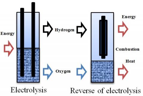
A FC converts the chemical energy directly into electrical energy and thus water and electricity are produced from oxygen and hydrogen and this without any thermal or mechanical process [15].
The principle of operation of a FC can be described as the reverse of the electrolysis of water. In fact, there is a controlled electrochemical combustion of hydrogen and oxygen, with a simultaneous production of electricity.
The FC comprises an anode and a cathode separated by an electrolyte which allows the migration of ions from one electrode to another under the effect of the created electric field.
The anode supplied with fuel (H2, CH3OH ...) is the seat of an oxidation reaction such as:
$2 H_{2} \rightarrow 4 H^{+}+4 e^{-}$ 0 Volts (7)
The cathode fed with oxidizer is the seat of a subsequent reduction reaction and the presence of a catalyst, usually platinum that accelerates the two half-reactions.
$O_{2}+4 H^{+}+4 e^{-} \rightarrow 2 H_{2} O \quad 1,23$ Volts (8)
Figure 4. Electrolysis-Reverse electrolysis
Figure 4 illustrates the difference between the phenomenon of electrolysis and that of reverse electrolysis.
The global real potential of the Proton Exchange Membrane Fuel Cells (PEMFC) is given by the equation:
$U_{P A C}=E_{\text {Nesrnst}}-V_{\text {act}}-V_{\text {ohn}}-V_{\text {conc}}$ (9)
The activation losses are given by the TAFEL equation:
$V_{a c t}=A \times \ln \left(\frac{I_{F C}+i_{n}}{i_{0}}\right)$ (10)
The ohmic losses with Rm total resistance of the FC:
$V_{o h m}=R_{m} \times\left(I_{F C}+I_{n}\right)$ (11)
The Concentrations losses:
$V_{\text {conc}}=-B \cdot \ln \left(1-\frac{I_{F C}+i_{n}}{i_{L}}\right)$ (12)
The chosen type is PEMFC using hydrogen as fuel and oxygen as oxidant. The total real potential of the PEMFC can be given by the following equation [15]:
$U_{P A C}=0,2817-0,85 \cdot 10^{-3}(T-298,15)$$+4,308.10^{-5} \times T \times\left[\ln \left(\frac{3}{4} \times P_{a no}\right)+\frac{1}{2} \ln \left(\frac{1}{2} \times P_{c a t}\right)\right]$
$+2.10^{-4} \ln A+B\left(1-\frac{J}{J_{\max }}\right)$$+4,3.10^{-3} \ln \left(\frac{0,75 \times P_{\text {ano}}}{1,09.10^{6} \exp \left(\frac{77}{T}\right)}\right)$
$+7,6.10^{-5} \times T \times \ln \left(\frac{0,5 \times P_{c a t}}{5,08.10^{-6} \exp \left(-\frac{498}{T}\right)}\right)$$+2,86.10^{-3}-I_{P A C} \times R c-1,93.10^{-4} I_{n} \times I_{P A C}$ (13)
$-\frac{181,6 \times I_{P A C}\left(1+0,03\left(\frac{I_{P A C}}{A}\right)+0,062\left(\frac{T}{303}\right)^{2}\left(\frac{I_{p a c}}{A}\right)^{2,5}\right)}{A\left(\lambda_{\frac{H_{2} O}{S O_{3}}}-0,638-3\left(\frac{I_{P A C}}{A}\right)\right) \times \exp \left(4,18\left(\frac{T-303}{T}\right)\right)}$
The dynamic behavior of the PEMFC can be represented by the following equivalent electrical circuit [15, 16].
Figure 5 explicitly translates relation 13 where in this equivalent circuit, the gap of the activation voltage represented by the resistance Ract, and the concentration voltage represented by the resistance Rcon is caused by the effect of the double layer charge.
Knowing that this phenomenon occurs when there is an accumulation of charges between two different materials that are in direct contact.
The charge layer in the electrode/electrolyte interface behaves like a capacitor.
Figure 5. Electrical equivalent circuit of a FC
3.1 Water flow
This is the amount of water that the pump can supply during a given interval of time. On pumping, the flow (Q) is usually given in litters per hour (l/h) or gallons per hour (g/h). For solar pumping, the flow is often expressed in cubic meter per day (m3/d) [14, 17].
$Q_{v}=v \times D$ (14)
where, Qv: Water flow, v: flow speed, D: pipe section.
3.2 Total dynamic head (TDH)
To convey a liquid, the pump should provide some pressure called TDH. This is the pressure difference in meters of water gauge (mwg) between the aspiration and discharge orifices.
We have to mention that more the TDH is great; the flow delivered by the pump becomes low. The expression of TDH is given by [14] :
$T D H=\left(H_{a}+H_{r}\right)+\left(J_{a}+J_{r}\right)+P_{r}$ (15)
Or even:
$T D H=H_{g}+J_{c}+P_{r}$ (16)
where, Ha: suction height, Hr: discharge height, Hg: geometric height, Ja: pressure losses at suction, Jr: pressure losses at discharge, Jc: pressure losses, Pr: discharge pressure.
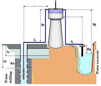
Figure 6. Pumping from a water reserve or borehole well
Figure 6 shows all the variables characterizing the basic data of the pump. The static level Ns of borehole well is the distance from the ground to the level of water in surface before pumping and the dynamic level Nd is the distance from the ground to the surface of the water when pumping to an average flow.
The drawdown Rm is the difference between dynamic level Nd and static level Ns.
There is a drawdown value where pumping should stop.
3.2.1 Suction height
The suction height in a pumping system is the vertical dimension measured between the surface of aspiration tank and the axis of the pump.
The theoretical value is 10.33 meters at the atmospheric pressure at sea level with water at 0℃.
This height can't be achieved, an attribute caused by cavitation and charge losses. In practice, this height is located around seven meters maximum at ambient temperature. In the event that this height is reached, it will be place an intermediate pump, put the reservoir on pressure or decrease the fluid temperature [18].
3.2.2 Geometric height
The geometric height can be defined as the sum of the suction height with that of the discharge in the case of a suction pump; ie Hg = Ha + Hr.
If the pump is placed on load, the suction height will be counted negatively; that is to say Hg = Hr - Ha.
In the case of an immersed pump, sunction height is equal zero, which means that Hg = Hr.
3.2.3 Pressure losses
The pressure losses are due to the friction of the liquid against the more or less smooth walls of the piping, to the changes in diameter, to the curves, to accessories such as tees, valves, elbows, etc.
The empirical formula of Darcy defines the pressure losses of a pipe and with equation 17; we can calculate the pressure losses at suction and the pressure losses at discharge [17].
$J_{c}=\frac{\lambda \times v^{2}}{2 \times g \times D}$ (17)
where, Jc: pressure losses, λ: pressure drop coefficient, v: average fluid speed, g: gravity, D: inside diameter of the pipe.
3.3 Pump characteristics
BRAUNSTEIN and KORNFELD introduced in 1981 the expression of mechanical power [16].
$P_{m e c}=K_{r} \times \omega_{r}^{3}$ (18)
The centrifugal pump opposes a resistant torque from which its expression is given by:
$T_{r}=K_{r} \times \omega_{r}^{2}+T_{s}$ (19)
According to the possible diameters of the wheels, the manufacturers supply curves of the flow rate Q as a function of TDH.
The model is identified by the expression of the TDH which is given by PELEIDER PETERMAN [14]:
$T D H=K_{0} \times \omega_{r}^{2}+K_{1} \times \omega_{r} \times Q-K_{2} \times Q^{2}$ (20)
The variation of the TDH as a function of the flow rate is a parabolic curve in which the point of intersection with the y-axis is the zero flow point. It is known as "wading point", where the valves are closed.
The pump power is calculated using the Bernoulli's theorem. The hydraulic energy is considered as the sum of the kinetic energy determined by the liquid movement in the tube and a stored potential energy, either in the form of an increase in pressure, or in the form of an increase in hill [17].
To provide water for drinking needs of a base camp located in desert areas which are not connected to power grids. In this hybrid pump station, a GPV and a FC are used as energy sources.
Before distributing it by gravity, the water is pumped into a water tank with a capacity V=75m3, similar to a battery, in a nominal flow (Qn= 15 m3/h) and ( TDH = 31m) [17, 18].
The pumping time is given by:
$T_{\text {pumping}}=V / Q_{n}=75 / 15=5$hours
4.1 FC sizing
In our application, the FC is expected to guarantee us DC bus voltage of the two inverters, i.e. 460 Volts. The dimensioning will be for a power of 3,500 Watts.
The voltage is dependent on the cells to be assembled in series, knowing that each cell provides between 0 and 1,1Volts.
On the other hand, the current is dependent on the total surface of a cell [15, 16].
For energy efficient of 60%, the working voltage is 0,63V/cell and the current density is 1.3 A/ cm².
The number of cells will therefore be:
$N_{\text {cell }}=\frac{460}{0.63}=730 \mathrm{cells}$
Then the current will therefore have a value of:
$I_{F C}=\frac{P}{U}=\frac{3500}{460}=7.60 A$
The surface of the FC will be:
$S_{F C}=\frac{7.60}{1,3}=5.85 \mathrm{~cm}^{2}$
4.2 GPV sizing
Dimensioning a GPV is an important step which, beforehand, must take into account all the variables, namely:
The photovoltaic generator power is:
$P_{g}=\frac{E_{c}}{T_{\text {pumping}}\left(1-\sum \text {losses}\right)}=\frac{P_{\text {del}}}{\left(1-\sum \text {losses}\right)}$ (21)
With "ålosses" is the sum of power losses caused by temperature and dust and representing about one-fifth of the power delivered by all modules.
Mechanical power "Pmec" is given by the manufacturer of centrifugal pumps and the hydraulic power required moving water from one point to another is:
$P_{H}=P_{\text {mес}} \times \eta_{\text {рumр}}=\rho \times g \times T D H \times Q_{V}$ (22)
where, $P_{H}=1000 \times 9.81 \times 30 \times \frac{15}{3600}=1226.25 \mathrm{~W}$
The electric power "Pelec" necessary for operation of the engine is:
$P_{\text {elec}}=\frac{P_{\text {mec}}}{\eta_{\text {motor}}}=\frac{P_{H}}{\eta_{\text {punp}} \times \eta_{\text {motor}}}$ (23)
The electric power actually applied, includes the consumption of the static converters used in the power chain:
$P_{d e l}=\frac{P_{\text {elec}}}{\eta_{\text {inverter}}}=\frac{P_{H}}{\eta_{\text {inverter}} \times \eta_{\text {pump}} \times \eta_{\text {motor}}}$ (24)
The electrical power also includes the consumption of static converters used.
In particular, the inverter having an efficiency of about 95%, the numeral application gives:
$P_{\text {del}}=\frac{1226.25}{0.95 \times 0.55 \times 0.89}=2636 \mathrm{~W}$
The necessary load power is evaluated by taking into account the daily pumping hours such as:
$E c=P_{\text {del}} \times T_{\text {Pumping}}=2636 \times 5=13180 \mathrm{Wh}$
Hence, the power of the PV generator is:
$P_{g}=\frac{P_{\text {del}}}{\left(1-\sum \text {losses}\right)}=\frac{2636}{1-0.2}=3295 \mathrm{~W}$
The required number of the Siemens SM 110-24 photovoltaic panel with "Ps" as standardized power is:
$N=\frac{P_{g}}{P_{s}}=\frac{3295}{110} \approx 30$ Panels
The results of sizing calculations presented in section 04 are shown in Table 2.
Table 2. Simulation parameters
|
Designation |
Value |
Designation |
Value |
|
Number of cells Ncell |
730 |
Delivered power Pdel |
2636 W |
|
Surface of cells SFC |
5.85 cm² |
Hydraulic power PH |
1226.25 W |
|
Pumping time |
5 hours |
Electric energy Ec |
13180 Wh |
|
photovoltaic panel N |
30 |
PV generator power Pg |
3295W |
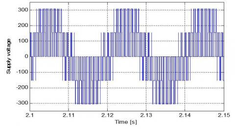
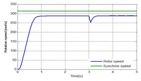
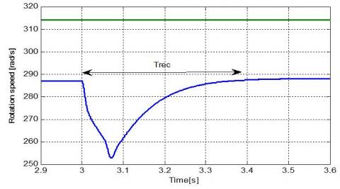
The voltage from the first arm of the inverter is shown in Figure 7. Figure 8 and Figure 9 shows DSIM rotation speed as a function of time. The zoom of the Figure 8 for the FC activation period is illustrated Figure 9.
One can note that the speed response is smooth with no overshoot. It is also clear from Figure 9 that the DSIM follows its reference speed which is equal to 288 rad/s with a steady state error which is neglected. When we switch from one source to another i.e. (PEMFC instead of PV), the motor speed drops from 287 rad/s to 226 rad/s and it recovers its driving speed in a recovery time Trec equal to 0.4 second.
Figure 7. Voltage va1 from inverter
Figure 8. Motor rotation speed
Figure 9. Motor rotation speed (Zoom)
Figure 10. Electromagnetic torque-Pump load torque
Figure 10 shows the DSIM electromagnetic torque and the pump load torque applied to it. It is clear from that figure that motor follows exactly the pump load torque with a hysteresis band equal to 4 N.m. Some fluctuations in the pump torque, resulting from a variation in the recorded sunshine, are also observed.
At start-up, the torque of the machine oscillates, reaching 28 Nm, before stabilizing, with some ripples, around a value of 12.5 Nm. The pump, in turn, opposes a resistant torque, which increases, rapidly, for a period of 0.8 s, before monitoring the evolution of the engine torque.
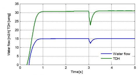
Figure 11 reveals the evolution of the water flow and the TDH. One can note from that figure that both of them have the same shape as the motor rotation speed.
It should be noted that, to have a flow rate in the pipes, it would be necessary to reach a certain speed of rotation obtains after few moments of star-up.
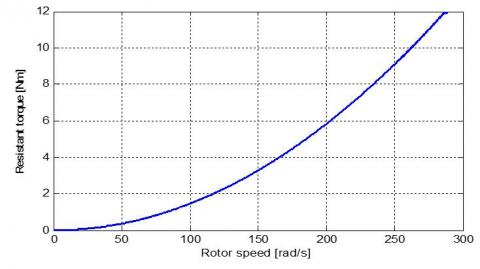
Figure 12 and Figure 13 confirm respectively the quadratic relation that exists between pump torque and its rotation speed (Eq. 19), TDH and rotation speed (Eq. 20).
Figure 11. TDH and water flow versus time
Figure 12. Resistant Torque vs Motor rotation speed
Figure 13. Dynamic head vs Motor rotation speed
From Figure 14 one can state that the pump will start pumping water if and only if the rotation speed is beyond the threshold speed which is equal in this work to 151 rad/sec. It is also worth noticing that the motor rotation speed and water flow are directly proportional.
The pump torque, rotation speed, pumped flow rate, and TDH are dependent on the variation in illumination. However, the use of the maximum power point search technique makes it possible to overcome the handicap of low illumination.
The need for a strong current at startup requires a coupling of the panels, in such a way, to have the sum of the currents, then to return to the coupling providing a voltage necessary for operation.
Figure 14. Water Flow vs Motor rotation speed
Hybrid pumping stations are now widely used to electrify isolated areas. They are likely to spread on a large scale, in the long term, to meet their energy needs.
The distribution of water by gravity avoids continuous pumping and the idea of using photovoltaic cells and fuel cells to fill a water tower is very beneficial and will replace traditional pumping systems even if the cost factor is significant at first, but it will be depreciated.
The idea of replacing conventional storage with a fuel cell seems to be more efficient and the use of a MASDE, as a motor driving the centrifugal pump, offers reliability and a possibility of operation in degraded mode.
|
DC/AC |
Inverter |
|
|
DC/DC |
Converter |
|
|
DSIM |
Dual stator induction motor |
|
|
FC |
Fuel cell |
|
|
GPV |
Photovoltaic generator |
|
|
mwg |
Meter of water gauge |
|
|
PEMFC |
Proton Exchange Membrane Fuel Cells |
|
|
PV |
Photovoltaic |
|
|
PWM |
Pulse with modulation |
|
|
A |
Tafel slope |
|
|
B |
mass transfer constant |
|
|
D |
Inside diameter of the conduit |
|
|
Enernst |
Unit cell thermodynamic potential |
|
|
fr |
Coefficient of friction |
|
|
g |
Gravity |
|
|
Ha |
Suction height |
|
|
Hd |
Set of linear and singular losses |
|
|
I |
Moment of inertia |
|
|
IFC |
Fuel cell current |
|
|
iL |
Limiting current for which all fuel is used. |
|
|
in |
Internal current |
|
|
ir,abc |
Rotor current |
|
|
i0 |
Exchange current |
|
|
i1,abc/ i2,abc |
Currents of star 1and star 2 |
|
|
J |
current density |
|
|
Jmax |
Maximum current density, A / cm² |
|
|
Ja |
Pressure losses at suction |
|
|
Jc |
Pressure drop in a pipeline |
|
|
Jr |
pressure losses at discharge |
|
|
Kr |
Proportionality coefficient |
|
|
Lx,y |
Mutual inductor |
|
|
n |
Ideality factor |
|
|
NS |
Static level |
|
|
Nd |
the dynamic level |
|
|
p |
Number of pole pairs |
|
|
Pmec |
Mechanical power |
|
|
Ps |
normalized power |
|
|
Pano |
Partial pressure of hydrogen, Atm |
|
|
Pcat |
Partial oxygen pressure, Atm |
|
|
Pr |
Discharge pressure |
|
|
Q |
Flow |
|
|
Rr |
Rotor resistor |
|
|
Rs |
Stator resistor |
|
|
Rsl |
Serial resistor |
|
|
Rm |
Drawdown |
|
|
Rsh |
Shunt resistor |
|
|
SFC |
FC surface |
|
|
TDH |
Total dynamic head |
|
|
Tem |
Electromagnetic torque |
|
|
Tr |
Resistant torque |
|
|
Tj |
Cell junction temperature |
|
|
Ts |
Static torque |
|
|
V1,abc |
Stator voltage of star 1 |
|
|
V2,abc |
Stator voltage of star 2 |
|
|
v |
fluid velocity |
|
|
Vact |
activation loss |
|
|
Vohm |
Ohmic losses |
|
|
Vconc |
Concentration loss |
|
|
Upac |
The overall real potential of the fuel cell |
|
|
wmag |
magnetic energy |
|
|
Wr |
Rotation speed |
|
|
Greek symbols |
||
|
ηinverter |
Inverter efficiency |
|
|
ηpump |
Pump efficiency |
|
|
ηmotor |
Motor efficiency |
|
|
θe, θm |
Electric & mechanical angle |
|
|
λ |
pressure loss coefficient |
|
|
ρ |
Volumic mass |
|
|
Ф1,abc |
Stator fluxes of star 1 |
|
|
Ф2,abc |
Stator fluxes of star 2 |
|
|
Фr,abc |
Rotor fluxes |
|
APPENDIX
(1) FC parameters.
|
Designation |
Value |
Designation |
Value |
|
A |
100 |
B |
16e-3 |
|
Jmax |
49,34375e-3 |
Lamda |
14 |
|
Rc |
1e-3 |
S |
5.85 |
|
Pano |
0.01 |
Pcat |
0.02 |
(2) Centrifugal pump parameters
|
Designation |
Value |
Designation |
Value |
|
Nominal speed ωn |
150 rad/s |
constant K0 |
4.9234.10-3 m.s²/rad² |
|
Nominal height |
12 m |
constant K1 |
1.5826.10-5 s²/(rad.m) |
|
Nominal flow |
21 m3/h |
constant K2 |
-18144 s²/m5 |
|
Efficiency |
55 % |
Pump inertia |
0.02 kg.m² |
(3) Photovoltaic panels SIEMENS SM 110-24
|
Designation |
Value |
|
Panel maximal power. |
POP =110 W |
|
Current at the maximum power point. |
IOP =3.15 A |
|
Voltage at the maximum power point. |
VOP =35 V |
|
Current of short circuit |
ICC =3.45 A |
|
Open circuit voltage |
VCO =43.5 V |
(4) Parameters of the DSIM
|
Designation |
Value |
Designation |
Value |
|
Nominal power |
4.5 kW |
Stator resistance |
Rs=3.72W |
|
Nominal voltage |
220 V |
Rotor resistance |
Rr=2.12 W |
|
Nominal current |
6.5 A |
Stator inductance |
Ls=0.022 H |
|
Efficiency |
89% |
Rotor inductance |
Lr = 0.006 H |
|
Number of poles |
2p=2 |
Mutual inductor |
Lm=0.3672 H |
|
Moment of inertia |
I=0.0625 kg.m² |
Coefficient of friction |
Kf =10-3 Nms/rd |
[1] Rekioua, D., Matagne, E. (2012). Optimization of Photovoltaic Power System: Modelization, Simulation And Control. Green Energy and Technology, Springer-Verlag London. https://doi.org/10.1007/978-1-4471-2403-0
[2] Mokrani, Z., Rekioua, D., Rekioua, T. (2014). Modelling, control and power management of hybrid photovoltaic fuel cells with battery bank supplying electric vehicle. International Journal of Hydrogen Energy, 39(27): 15178-15187. https://doi.org/10.1016/j.ijhydene.2014.03.215
[3] Kaabeche, A., Belhamel, M., Ibtiouen, R., Moussa, S., Benhaddadi, M.R. (2006). Optimisation d’un système hybride éolien–photovoltaïque totalement autonome. Renewable Energy Journal, 9(3): 199-209.
[4] Hachemi, A. (2017). Modélisation énergétique et optimisation économique d'un système hybride dédié au pompage. PhD in Hydraulics, University Mohamed Khider of Biskra.
[5] Gergaud, O., Multon, B., Benahmed, H. (2002). Analysis and experimental validation of varios photovoltaic system models. 7th International Electrimacs Congress, Montréal.
[6] Zarour, L. (2010). Etude technique d’un système d’énergie hybride photovoltaique-eolien hors réseau. Doctorat en électrotechnique, University Mentouri Constantine.
[7] Belatel, M., Benchikh, F., Simohamed, Z., Ferhat, F., Aissous, F.Z. (2011). Technologie du couplage d’un système hybride de type photovoltaïque-éolien avec la pile à combustible pour la production de l’électricité verte. Revue des Énergies Renouvelables, 14(1): 145-162.
[8] Gailly, F. (2011). Alimentation électrique d'un site isolé à partir d'un générateur photovoltaïque associé à un tandem électrolyseur / pile à combustible (batterie H2/O2). École Doctorale Génie Électrique, Électronique et Télécommunications : du système au nanosystème.
[9] Hadiouche, D., Razik, H., Rezzoug, A. (2000). Study and simulation of space vector PWM control of double-star induction motors. International Power Electronics Congress - CIEP, Acapulco, Mexico, Mexico, pp. 42-47. https://doi.org/10.1109/CIEP.2000.891389
[10] Umesh, B.S., Sivakumar, K. (2016). Dual-inverter-fed pole-phase modulated nine-phase induction motor drive with improved performance. IEEE Transactions on Industrial Electronics, 63(9): 5376-5383. https://doi.org/10.1109/TIE.2016.2561268
[11] Muhsen, D.H., Khatib, T., Nagi, F. (2017). A review of photovoltaic water pumping system designing methods, control strategies and field performance. Renewable and Sustainable Energy Reviews, 68(1): 70-86. https://doi.org/10.1016/j.rser.2016.09.129
[12] Rekioua, D., Bensmail, S., Bettar, N. (2014). Development of hybrid photovoltaic-fuel cell system for stand-alone application. International Journal of Hydrogen Energy, 39(3): 1604-1611. https://doi.org/10.1016/j.ijhydene.2013.03.040
[13] García, P., Torreglosa, J.P., Fernández, L.M., Jurado, F. (2013). Optimal energy management system for stand-alone wind turbine / photovoltaic / hydrogen / battery hybrid system with supervisory control based on fuzzy logic. International Journal of Hydrogen Energy, 38(33): 14146-14158. https://doi.org/10.1016/j.ijhydene.2013.08.106
[14] Taner, T. (2018). Energy and exergy analyze of PEM fuel cell: A case study of modeling and simulations. Energy, 143: 284-294. https://doi.org/10.1016/j.energy.2017.10.102
[15] Yu, D., Yuvarajan, S. (2005). Electronic circuit model for proton exchange membrane fuel cells. Journal of Power Sources, 142(1-2): 238-242. https://doi.org/10.1016/j.jpowsour.2004.09.041
[16] Amrouche, F., Mahmah, B., Belhamel, M., Benmoussa, H. (2005). Modelling of a fuel cell PEMFC fed directly with hydrogen-oxygen and experimental validation. Review of Renewable Energy, 8: 109-120.
[17] Mebarki, N., Rekioua, T., Mokrani, Z., Rekioua, D., Bacha, S. (2016). PEM fuel cell/ battery storage system supplying electric vehicle. International Journal of Hydrogen Energy, 41(45): 20993-21005. https://doi.org/10.1016/j.ijhydene.2016.05.208
[18] Arrouf, M. (2007). Optimisation de l'ensemble onduleur, moteur et pompe branché sur un générateur photovoltaique. PhD in Electronics, Constantine.