Tao Zhang* | Qiang Hao | Zheng Zheng | Chuang Lu
© 2020 IIETA. This article is published by IIETA and is licensed under the CC BY 4.0 license (http://creativecommons.org/licenses/by/4.0/).
OPEN ACCESS
As a novel voltage control device, electric spring (ES) can effectively suppress the voltage fluctuations across critical loads (CLs), and solve the various problems with electrical quality induced by the grid access of renewable energy resources (RES). However, the traditional controllers for the ES system can no longer meet the control requirements, as the environment is complicated by the growing number of load-side nonlinear loads and uncertain disturbances. To solve the problem, this paper proposes a control system based on finite control set-model predictive control (FCS-MPC), and applies it to the ES. Firstly, a load-side circuit prediction model was established and analyzed. Next, a control system was designed based on FCS-MPC. Finally, the proposed system was proved feasible and effective through MATLAB/Simulink simulation and dSPACE physical experiment. The results show that the proposed FCS-MPC system can directly control the ES, easily handle system constraints, achieve robust dynamic and static performance, eliminating the need for pulse width modulation (PWM).
electric spring (ES), finite control set-model predictive control (FCS-MPC), voltage fluctuation, power quality
The development of renewable energy sources (RES) has accelerated the reform of the energy structure. However, the intermittency and unsustainability of RES have brought various power quality problems to the power supply and distribution network [1, 2]. Proposed by Hui et al. [3], electric spring (ES) provides a new solution to such problems. Unlike the traditional circuit compensation device, the ES operates in a distributed manner on the load side, making the power consumption more reliable on the load side [4]. Compared with the static var compensator (SVC), the ES boasts small capacity and high reliability [5]. Different from the traditional measures to alleviate RES supply fluctuations (e.g. controlling load switches), the ES improves the comfort and happiness of power users, without hindering the normal power consumption on the load side [6].
The original ES structure can only realize reactive power compensation: the device is connected in series with the non-critical loads (NCLs), which are insensitive to voltage changes, forming smart loads (SLs); then, the ES transfers the voltage fluctuations on the bus to the NCLs, thereby stabilizing the bus voltage. In this way, the voltage of the critical loads (CLs) on the bus, which are sensitive to voltage changes, will also be stabilized. Through years of research, the ES has been proved to be feasible in frequency stabilization, power factor correction, and filtering [7, 8].
Over the years, the ES control has become increasingly robust, nonlinear, and intelligent. The control devices have evolved from the proportional-integral (PI) controller suitable for ES-1 topology [9, 10], to quasi-proportional resonant (PR) controller for ES-2 topology [11], and to intelligent controllers like fuzzy controller [12]. The increase of nonlinear loads, coupled with various circuit interferences, raise stricter requirements on the normal operation of the ES. In alternative current (AC) ES control system, the PI controller cannot achieve error-free tracking of the AC reference signal, and the parameter debugging of the traditional linear controller is time-consuming and laborious. To solve the problem, more and more nonlinear control theories have been proposed and applied to inverter systems, such as hysteresis control, sliding mode control, repetitive control, and adaptive control [13].
Model predictive control (MPC) is an algorithm that uses the system model to predict the controlled quantity and approximate it to the reference quantity [14]. The algorithm supports fast dynamic response and transient response, and adapts well to nonlinear constraints. However, the MPC theory was not widely accepted at the beginning, because the control system needs a high-performance hardware platform to perform the numerous calculations in each sampling period. Thanks to the development of computer technology, the MPC has become a research hotspot in the control of power electronic converters [15, 16]. For instance, the finite control set-model predictive control (FCS-MPC) [17, 18] can achieve flexible and multivariable control, eliminating the need for pulse width modulation (PWM) of the output. It is suitable for nonlinear systems with constraints. Previous studies [19, 20] have confirmed the feasibility of the MPC in the control of single-phase and three-phase grid-connected inverters. Unlike other control methods, the MPC takes the predicted circuit quantities in future as the reference for the current actions of the system.
This paper introduces the FCS-MPC into ES control system, with the aim to improve the anti-interference ability of the ES and to optimize the dynamic and static ES performance under complex load environment. Firstly, a load-side circuit prediction model was established and analyzed. On this basis, the prediction formula of ES output voltage and the calculation formula of ES reference formula were created, as well as the performance indicator function. Finally, the proposed control strategy was proved feasible and effective through MATLAB simulations and dSPACE physical experiments, and the simulation and experimental results were given in the presence of interference in the circuit.
Figure 1 shows the structure of the ESs connected to the power system, where Z0, Z1, and Z2 are the impedances of the transmission line. On the supply side, there is a RES and a grid supply. On each load unit, there is an SL made up of an ES serial-connected with an NCL. Each SL is connected in parallel with the CL into a load unit. When the RES power supply fluctuates, the ESs of all load units on the line participate in the regulation. The failure of a single ES does not affect the stability of the bus voltage, providing a guarantee for the reliability of power consumption.
Figure 1. The structure of the ESs connected to the power system
The topologies and functions of ES-1 to ES-7 are introduced in details by Wang et al. [21]. Among them, ES-2 topology is selected for this research. ES-2 topology is extended from ES-1 topology by adding a battery on the direct current (DC) side, achieving the new function of power consumption [22, 23].
Figure 2 is the simplified model of a single ES load unit and the supply side, whereUg is the supply-side voltage, Zt is the transmission line impedance, Ut is the transmission line voltage drop, It is the bus current, Zcl and Zncl are respectively the impedances of CL and NCL, and Ucl and Uncl are respectively the voltages of CL and NCL.
Figure 2. The topology of a single load unit
The ES-2 circuit topology is given in the red dotted box, where S1~S4 are switching tubes, L and C are respectively the inductance and capacitance of the low-pass filter, UC is the output voltage of ES, Vin is the battery voltage on the DC side of the inverter bridge, Q is the ES switch, and Tri is the switch signal.
When a compensation demand arises in the circuit, the Tri signal disconnects Q, so that ES and NCL are connected in series. Then, the controller collects the circuit quantities, and calculate the control signal to act on S1~S4. Through the control, the DC is inverted to AC, and the ES generates the output voltage, making the bus voltage stable. When the ES is needed for circuit regulation, Q is closed to short-circuit ES.
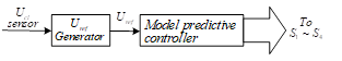
This paper constructs a control system based on the ES system model (Figure 3). The principle of the control system goes as follows: the CL reference voltage Uref is generated based on the CL voltage Ucl collected by the voltage sensor, and imported to the MPC to output a control signal for switch tubes S1~S4 on the inverter bridge; through the control, the output voltage of the ES UC approaches the reference voltage UCref, that is, the error between the two voltages is minimized.
Figure 3. The block diagram of our control system
The performance indicator function, which is often adopted in prediction models, measures the optimization trend of system indices. In MPC rolling optimization, the function is the key player that decides the controller output, and the enabler of the MPC to solve multivariable constrained problems. To simplify the control structure and reduce the calculation amount of the control system, the square of the difference gmin between UCref and the predicted value was selected as the performance indicator function:
${{\text{g}}_{min}}\text{=}{{\left( {{U}_{Cref}}\left( k+1 \right)-{{\overset{\wedge }{\mathop{U}}\,}_{C}}\left( k+1 \right) \right)}^{2}}$ (1)
The calculation of gmin depends heavily on three parameters: the CL reference voltage Uref, the predicted ES output voltage $\widehat{U}_{c}(k+1)$ , and the reference value of the output voltage UCref. Therefore, the calculation process of the three parameters is detailed below.
3.1 Generation of Uref
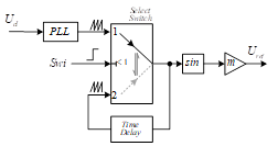
The Uref was generated by the method shown in Figure 4, for the stability of the amplitude and phase of CL voltage.
When ES is not needed for circuit regulation, the Swi signal is set to low level, and the Tri signal (Figure 2) to high level. Then, switch Q is closed, the voltage sensor collects Ucl, and the phase of Ucl is obtained through the phase-locked loop. Next, channel 1 in the switch is selected for signal transmission, and the phase is passed through the sin module and booster m to generate the CL reference voltage Uref. But Uref has not effect at this time.
When ES is needed for circuit regulation, the Swi signal is set to high level, channel 2 in the switch is selected for signal transmission, and the Tri signal is set to low level. Then, switch Q is opened, and ES is connected in parallel to the bus. The phase signal of Uref will change periodically after passing the time delay module. The delay is an integer number of power frequency cycles.
The Uref generation method in Figure 4 keeps Uref unchanged regardless of circuit conditions, eliminates the interference of external factors on CL, and minimizes the dependence on external circuit parameters, thereby improving the robustness of our control system.
Figure 4. The structure of Uref generator
3.2 Prediction of $\widehat{U}_{C}(k+1)$
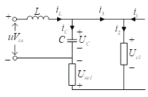
To analyze the load-side model, Figure 2 was further simplified in the ES working state into Figure 5, where i1 is the current input to a single load unit on the bus, i2 is the CL current, Ucl is the CL voltage, i3 is the SL current, iL and ic are respectively the inductance and capacitance currents of the filter, Uc is the ES output voltage, Uncl is the NCL voltage, uVin is the inverter bridge output voltage, with u being the switching function. If u=1, S1 and S4 (Figure 2) are closed; if u=0, S1 and S2 are closed, or S3 and S4 are closed; if u=-1, S2 and S3 are closed.
Figure 5. The simplified structure of the load side during ES operation
To reduce the influence of the sensor in the circuit on the predicted value, this paper only collects the inductor L current and the capacitor C voltage to predict the ES output voltage:
$L\frac{d{{i}_{L}}}{dt}=u{{V}_{in}}-{{U}_{C}}$ (2)
$C\frac{d{{U}_{C}}}{dt}={{i}_{L}}-{{i}_{3}}$ (3)
Let Ts be the discrete sampling period of the ES control system. From formula (2) and the forward difference formula [24], the current of the inductor L at time k can be predicted by:
${{\overset{\wedge }{\mathop{i}}\,}_{L}}(k)={{i}_{L}}(k-1)+\frac{Ts}{L}(u{{V}_{in}}(k)-{{U}_{C}}(k))$ (4)
From formula (3) and backward difference formula [25], the ES output voltage at time k+1 can be predicted by:
${{\overset{\wedge }{\mathop{U}}\,}_{C}}\left( k+1 \right)={{U}_{C}}\left( k \right)+\frac{Ts}{C}\left( {{\overset{\wedge }{\mathop{i}}\,}_{_{L}}}\left( k \right)-{{\overset{\wedge }{\mathop{i}}\,}_{3}}\left( k \right) \right)$ (5)
For convenience, it is assumed that i3 does not change in a sampling period Ts:
${{\overset{\wedge }{\mathop{i}}\,}_{3}}(k)\approx \overset{\wedge }{\mathop{{{i}_{3}}}}\,(k-1)$ (6)
From formula (3), formula (6), and forward difference formula [24], we have:
$\overset{\wedge }{\mathop{{{i}_{3}}}}\,(k-1)\text{=}{{i}_{L}}(k-1)-\frac{C}{Ts}\left( {{U}_{C}}\left( k \right)-{{U}_{C}}\left( k-1 \right) \right)$ (7)
Substituting formulas (4), (6), and (7) into formula (5), we have:
${{\overset{\wedge }{\mathop{U}}\,}_{C}}\left( k+1 \right)\text{=}\frac{T{{s}^{2}}}{LC}u{{V}_{in}}\left( k \right)+\left( 2-\frac{T{{s}^{2}}}{LC} \right){{U}_{C}}\left( k \right)-{{U}_{C}}\left( k-1 \right)$ (8)
3.3 Calculation of UCref
To eliminate the interference of bus current $i_{1}$ on the system, the output voltage control was adopted, with the controlled quantity being volage Uc. When the supply side fluctuates, the bus current changes accordingly. To stabilize Ucl, the amplitude and phase of ES output voltage will both change. The controlled quantity can be derived from the circuit in Figure 5:
${{U}_{C}}\text{=}{{U}_{cl}}+{{U}_{ncl}}$ (9)
Substituting current i1, and load parameters Zncl and Zcl into formula (9), the reference value UCref of ES output voltage UC at time k+1 can be expressed as:
${{U}_{Cref}}\left( k+1 \right)=\left( 1+\frac{{{Z}_{ncl}}}{{{Z}_{cl}}} \right){{U}_{ref}}\left( k+1 \right)-{{Z}_{ncl}}{{i}_{1}}\left( k+1 \right)$ (10)
where, Uref is the reference voltage of CL, whose effective value remains constant; i1 is the current flowing from the bus into the load side, which changes in real time under the effects of changes on both supply side and load side. UCref also changes in real time.
Before calculating UCref by formula (10), it is necessary to obtain the values of i1 and Uref at time k+1. Since the change of Uref is periodic, and i1 is collected from the circuit, it is assumed that i1 does not change between two adjacent sampling periods:
${{i}_{1}}\left( k+1 \right)\approx {{i}_{1}}\left( k \right)$ (11)
The i1 value at time k was measured by installing a current sensor on the outside of the load unit. The calculation method of i1 in formula (10) enhances the anti-interference ability of the control system, and optimizes the dynamic performance of the system under supply-side fluctuations.
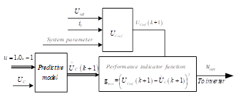
As shown in Figure 6, the FCS-MPC control system first derives UCref(k+1) and UC from Uref, i1, and circuit parameters. Then, the $\widehat{U}_{C}(k+1)$ value is predicted from these results and the switching function states u of full-bridge inverter of the ES. Coupling the predicted result with the performance indicator function, the optimal value uopt is directly applied to generate the driving signal. The uopt does not need to be modulated.
Figure 6. The block diagram of the FCS-MPC control system
In this paper, the ES full-bridge inverter (Figure 2) is regarded as a nonlinear discrete system with 4 different vectors. The gate signals K1 and K2 can be defined as:
$\begin{align} & {{K}_{1}}\text{=}\left\{ \begin{matrix} 1 & {{S}_{1}}\text{ }is\text{ }opened\text{ }and\text{ }{{S}_{3}}\text{ }is\text{ }closed. \\0 & {{S}_{1}}\text{ }is\text{ }closed\text{ }and\text{ }{{S}_{3}}\text{ }is\text{ }opened. \\\end{matrix} \right. \\& {{K}_{2}}\text{=}\left\{ \begin{matrix} 1 & {{S}_{2}}\text{ }is\text{ }opened\text{ }and\text{ }{{S}_{4}}\text{ }is\text{ }closed. \\0 & {{S}_{2}}\text{ }is\text{ }closed\text{ }and\text{ }{{S}_{4}}\text{ }is\text{ }opened. \\\end{matrix} \right. \\\end{align}$ (12)
The switch states and output voltages are shown in Table 1. The output voltage has three states: +Vin, 0, and -Vin. In each sampling period, the control system needs to calculate the values of the performance indicator function under the three states. Then, the u value corresponding to the minimum value is taken as the ontroller output.
Table 1. The switch states and voltage vectors
|
K1 |
K2 |
u |
Output voltage |
|
0 |
0 |
0 |
0 |
|
1 |
0 |
1 |
+Vin |
|
1 |
1 |
0 |
0 |
|
0 |
1 |
-1 |
-Vin |
In each sampling period, the process in Figure 4 is implemented once. After the optimal output is obtained and transmitted to the inverter bridge, the sampling and calculation will be repeated in the next sampling period. Since the control system always looks for the switch state that makes the predicted value approach the reference value, Uc continues to approximate UCref, that is, Ucl continues to approach Uref. This control method minimizes the influence of change of bus current i1 over the load unit, and exhibits a certain anti-interference ability.
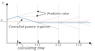
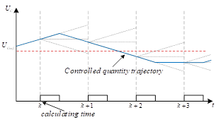
In ideal conditions, the entire control process, from sampling, calculation, decision-making to generating the output voltage, is completed in an instant, that is, the control time tends to infinitesimal. Figure 7 shows the variation of the controlled quantity with the reference value in ideal conditions. In the actual situation, however, it takes a certain time for the system to complete the control process. Figure 8 presents the variation of the controlled quantity with the reference value in the actual situation.
Figure 7. The trajectory of the controlled quantity in ideal conditions
Figure 8. The trajectory of the controlled quantity in actual situation
As shown in Figure 7, sampling, calculation, decision-making, and control were completed simultaneously in ideal conditions, and the controlled quantity could be stabilized in the shortest possible time. As shown in Figure 8, the entire control process was delayed by a calculation cycle, because the calculation consumed a certain amount of time. In the actual situation, the controlled quantity oscillated near the reference value, making the system unstable. To mitigate the negative impact of calculation time, this paper simplifies the structure of the control system to the maximum extent. Therefore, the calculation-induced delay in our system can be neglected. Moreover, the calculation time of our system can fully meet the requirements on the dSPACE physical experiment platform.
5.1 Simulation and result analysis
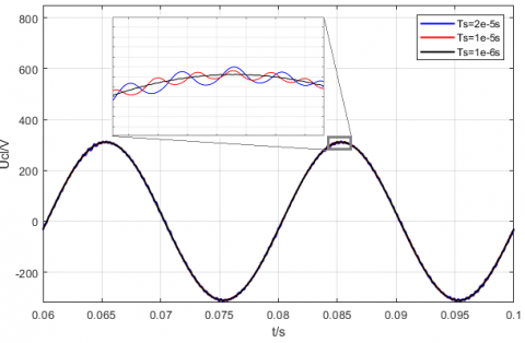
To verify the proposed FCS-MPC control system for the ES, a simulation model was established on MATLAB/Simulink to simulate the control effect of the system. The simulation circuit was built in accordance with Figure 2. The circuit parameters and controller parameters are listed in Table 2. Considering the effects of the sampling period on the quality of the controlled quantity in discrete sampling, the simulation was carried out under different sampling periods: 2e-5s, 1e-5s, and 1e-6s. The Ucl values under these periods are compared in Figure 9.
Table 2. The hardware parameters of the simulation circuit
|
Parameter |
Value |
|
Transmission line impedance Zt |
0.6Ω+2.86mH |
|
CL Zcl |
40Ω |
|
NCL Zncl |
4Ω |
|
Filter inductance L |
3.6mH |
|
Filter capacitance C |
100μF |
|
Battery voltage Vin |
360V |
Figure 9. The comparison of Ucl under different sampling periods
As shown in Figure 9, the shorter the sampling period, the smaller the fluctuation of the controlled quantity, and the closer the waveform is to the ideal sine. Because the MPC has no modulation link, the trigger pulse frequency it generates depends entirely on the discrete sampling period of the system. The shorter the sampling period, the higher the accuracy of the prediction result, and the faster the CL will enter the normal working environment in terms of electrical energy. Repeated simulations show that the proposed control system achieved fast calculation speeds under all three sampling periods, and experienced virtually no delay. As a result, the minimum sampling period of 1e-6s was adopted for subsequent simulation.
5.1.1 Simulation at 220V
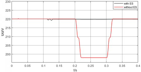
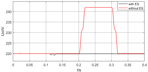
The next step is to verify whether the ES in the FCS-MPC control system could stabilize the CL voltage quickly and stably. Hence, the amplitude and effective value of Ucl were observed under the drop and rise of supply-side voltage, respectively. After debugging in MATLAB simulation, it is learned that the load-side load voltage is 220V, when the supply-side voltage Ug is 262V, under the circuit parameters in Table 2. Then, the supply-side voltage Ug was decreased and increased by 10% to 235.8V and 288.2V, respectively, and maintained for 0.1s. The simulation time was set to 0.4s. The time variations of Ug and Tri signal are recorded in Table 3.
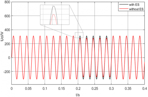
As shown in Table 3, the supply-side voltage remained normal in 0~0.2s, and resumed the normal state in 0.3~0.4s after the voltage dropped or rose in 0.2~0.3s. Figures 10 and 11 present the variations in Ucl amplitude during voltage drop and voltage rise, respectively. It can be seen that, when supply-side voltage fluctuated, the Ucl amplitude in the circuit with ES remained basically unchanged in 0~0.5s, ensuring the stable and good power environment at both ends of Zcl; the Ucl amplitude in the circuit without ES fluctuated significantly in 0.2~0.3s.
Table 3. The time variations of Ug and Tri signal
|
Time/s |
Ug/V |
Tri |
|
0~0.1 |
262 |
1 |
|
0.1~0.2 |
262 |
0 |
|
0.2~0.3 |
235.8 (drop)/288.2 (rise) |
0 |
|
0.3~0.4 |
262 |
0 |
Figure 10. The Ucl amplitude at the drop of supply-side voltage
Figure 11. The Ucl amplitude at the rise of supply-side voltage
Figures 12 and 13 display the variations in the effective value of Ucl during voltage drop and voltage rise, respectively. It can be observed that the effective value of Ucl in the circuit with ES fluctuated slightly after 0.1s, and then stabilized quickly at the reference value, owing to the sudden switching of the ES. When the supply-side voltage fluctuated, the Ucl always remained stably at about 220V, regardless of the voltage drop or rise in the circuit with ES, providing a stable and reliable power environment for Zcl. By contrast, the effective value of Ucl in the circuit without ES fluctuated with the supply-side voltage. Overall, the ES under FCS-MPC performs excellently in stabilizing Ucl voltage during voltage rise and voltage drop, which demonstrates the feasibility of the FCS-MPC control system and its strong adaptability to voltage fluctuations.
Figure 12. The effective value of Ucl at the drop of supply-side voltage
Figure 13. The effective value of Ucl at the rise of supply-side voltage
5.1.2 Simulation at 30V
To facilitate the comparison between the simulation results and the experimental results, a MATLAB simulation was carried out at a low voltage (30V), with basically the same circuit and controller settings as the simulation at 220V. The only difference is that the battery voltage Vin was changed from 360V to 48V, and the $U_{\text {ref}}$ was reduced from 220V to 30V. The supply-side voltage was also increased and decreased for the simulation.
Through debugging, it is learned that the CL voltage Ucl remained at 30V, when the ES was not involved in circuit regulation and the supply-side voltage Ug was set to 35.69V. Therefore, the supply-side voltage was decreased and increased by 10% to 32.04V and 39.16V. The simulation time was set to 0.5s. The time variations of Ug and Tri signal are recorded in Table 4.
Table 4. The time variations of Ug and Tri signal
|
Time/s |
Ug/V |
Tri |
|
0~0.1 |
35.69 |
1 |
|
0.1~0.2 |
35.69 |
0 |
|
0.2~0.3 |
32.04 (drop) |
0 |
|
0.3~0.4 |
39.16 (rise) |
0 |
|
0.4~0.5 |
35.69 |
0 |
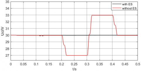
Figures 14 and 15 compare the amplitudes and effective values of Ucl in circuits with and without ES, respectively. In 0~0.1s, the supply-side voltage was normal, the Tri signal was 1, and the switch Q was closed, i.e. the ES was out of service. At 0.1s, the Tri signal was 0, and the switch Q was opened, i.e. the ES was put into use.
As shown in Figure 14, the Ucl amplitude in the circuit without ES fluctuated with the dropping or rising voltage, while that in the circuit with ES remained stable. As shown in Figure 15, the circuit with ES achieved a good performance in voltage stabilization. Regardless of voltage drop or voltage rise, the circuit quickly stabilized the effective value of Ucl near 30V. This proves the robustness and adaptability of the ES under the control of FCS-MPC.
Figure 14. The variations in Ucl amplitude at the drop or rise of supply-side voltage
Figure 15. The variations in the effective value of Ucl at the drop or rise of supply-side voltage
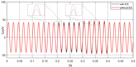
Figure 16 compares the phases of Ucl and UES at 30V. In 0~0.1s, the Tri signal was 1, and the switch Q was closed, i.e. the ES was out of service. In this case, the ES voltage output was 0. At 0.1s, the Tri signal was 0, and the switch Q was opened, i.e. the ES was put into use. At 0.2s, the supply-side voltage dropped. In 0.2-0.3s, the UC lagged Ucl by about 90°; the ES worked in capacitive mode under the voltage drop, and injected negative reactive power into the bus to stabilize the voltage across Zcl. In 0.3-0.4s, the supply-side voltage increased, and the grid voltage exceeded the reference value; in this case, the UC led Ucl by about 90°; the ES worked in capacitive mode under the voltage rise, and injected positive reactive power into the bus to stabilize the voltage across $Z_{c l}$. The above results further confirm the correctness and effectiveness of our control system.
Figure 16. The phase comparison between Ucl and UES
5.2 Physical experiment and result analysis
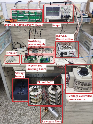
Figure 17 illustrates the physical experiment platform. For the safety of physical experiment, four 12V/24Ah batteries were connected in series to simulate the 48V DC power supply. The supply-side power source of the grid was simulated with a voltage regulator, with the effective value of Uref at 30V. The control part was simulated with a dSPACE DS1202 controller. The CL and NCL were simulated by adjustable resistors. The controller parameters in dSPACE were kept consistent with those in the simulation at 30V, except that the step length was adjusted to 5e-5s. To prevent short circuiting, the PWM dead time of the controller output was set to a sampling period.
Figure 17. The dSPACE-based ES experimental platform
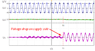
Figure 18. The waveforms of Ucl amplitude, Ucl effective value, and UC at voltage drop
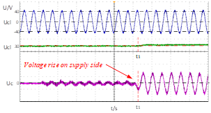
Figure 19. The waveforms of Ucl amplitude, Ucl effective value, and UC at voltage rise
Figures 18 and 19 compare the Ucl amplitudes, Ucl effective values, and UC as the supply-side voltage dropped or increased at time t1, respectively. It can be seen that Ucl amplitude did not fluctuate greatly, while the effective value of Ucl stabilized quickly after slight volatility, during the fluctuations of the supply-side voltage.
The ES was put into use after the switch Q was opened, and started to regulate the circuit at time t1. During ES regulation, the UC lagged Ucl at the drop of supply-side voltage, but led Ucl at the increase of supply-side voltage. This is because, the ES worked in capacitive mode under the voltage drop, and injected negative reactive power into the bus to stabilize the voltage across Zcl; the ES worked in capacitive mode under the voltage rise, and injected positive reactive power into the bus to stabilize the voltage across Zcl.
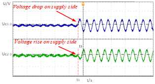
To clearly observe the ES working states at different voltage fluctuations, the UC phases at the drop and rise of supply-side voltage are compared in Figure 20. As the supply-side voltage started to fluctuate at time t1, there was a 180° difference between the UC phases at the drop and rise of supply-side voltage. The reason is that the UC lagged Ucl by 90° at voltage drop, but led the latter by 90° at voltage rise. The above analysis shows that the results of physical experiment agree with the simulation results. This further proves the feasibility and effectiveness of our control system.
Figure 20. The UC phases at the drop and rise of supply-side voltage
With the growing number of nonlinear loads in the circuit, in AC ES control system, the conventional PI controller cannot achieve error-free tracking of the AC reference signal, and the parameter debugging of the traditional linear controller is time-consuming and laborious. In this paper, the FCS-MPC is applied to the ES to solve the problem. After analyzing the model of the ES system, the authors derived the reference voltage of CL, the reference value of ES output voltage, and the predicted value of ES output voltage. On this basis, a control system was designed based on FCS-MPC. Then, the proposed control system was proved effective and correct through simulation on circuits at 220V and 30V. Finally, physical experiment was conducted to manifest the application prospects of the proposed method. The research results provide a good reference for the engineering application of FCS-MPC.
This work was supported in part by Henan mine power electronics device and control innovative technology team (Grant No.: CXTD2017085), Science and Technology Planning Project of Henan Province of China (Grant No.: 202102210295) and the Doctoral Scientific Research Foundation of Henan Polytechnic University (Grant No.: B2017-20).
[1] Guo, Y., Wang, Q., Yu, J. (2019). Assessment of voltage fluctuations based on wind power fluctuation characteristics. 8th Renewable Power Generation Conference (RPG 2019), Shanghai, China, pp. 1-6. https://doi.org/10.1049/cp.2019.0402
[2] Cheng, M., Zhu, Y. (2014). The state of the art of wind energy conversion systems and technologies: A review. Energy Conversion and Management, 88: 332-347. https://doi.org/10.1016/j.enconman.2014.08.037
[3] Hui, S.Y., Lee, C.K., Wu, F.F. (2012). Electric springs—A new smart grid technology. IEEE Transactions on Smart Grid, 3(3): 1552-1561. https://doi.org/10.1109/TSG.2012.2200701
[4] Yan, S., Luo, X., Tan, S.C., Hui, S.R. (2015). Electric springs for improving transient stability of micro-grids in islanding operations. In 2015 IEEE Energy Conversion Congress and Exposition (ECCE), pp. 5843-5850. https://doi.org/10.1109/ECCE.2015.7310480
[5] Che, X., Wei, T., Huo, Q., Jia, D. (2014). A general comparative analysis of static synchronous compensator and electric spring. In 2014 IEEE Conference and Expo Transportation Electrification Asia-Pacific (ITEC Asia-Pacific), pp. 1-5. https://doi.org/10.1109/ITEC-AP.2014.6940991
[6] Mohsenian-Rad, A.H., Leon-Garcia, A. (2010). Optimal residential load control with price prediction in real-time electricity pricing environments. IEEE Transactions on Smart Grid, 1(2): 120-133. https://doi.org/10.1109/TSG.2010.2055903.
[7] Yang, Y., Tan, S.C., Hui, S.Y. (2016). Voltage and frequency control of electric spring based smart loads. In 2016 IEEE Applied Power Electronics Conference and Exposition (APEC), pp. 3481-3487. https://doi.org/10.1109/APEC.2016.7468368
[8] Soni, J., Panda, S.K. (2017). Electric spring for voltage and power stability and power factor correction. IEEE Transactions on Industry Applications, 53(4): 3871-3879. https://doi.org/10.1109/TIA.2017.2681971
[9] Areed, E.F., Abido, M.A. (2015). Design and dynamic analysis of electric spring for voltage regulation in smart grid. In 2015 18th International Conference on Intelligent System Application to Power Systems (ISAP), pp. 1-6. https://doi.org/10.1109/ISAP.2015.7325565
[10] Lee, C.K., Tan, S.C., Wu, F.F., Hui, S.Y.R., Chaudhuri, B. (2013). Use of Hooke's law for stabilizing future smart grid—The electric spring concept. In 2013 IEEE Energy Conversion Congress and Exposition, pp. 5253-5257. https://doi.org/10.1109/ECCE.2013.6647412.
[11] Wang, Q., Cheng, M., Chen, Z., Wang, Z. (2015). Steady-state analysis of electric springs with a novel δ control. IEEE Transactions on Power Electronics, 30(12): 7159-7169. https://doi.org/10.1109/TPEL.2015.2391278
[12] Zhang, T., Lu, C., Zheng, Z. (2020). Adaptive fuzzy controller for electric spring. European Journal of Electrical Engineering, 22(3): 233-239. https://doi.org/10.18280/ejee.220304
[13] Yin, F.G., Wang, C. (2019). Review of electric spring: principle, topologies, control and applications. Power System Technology, 43(1): 174-184. https://doi.org/10.13335/j.1000-3673.pst.2018.2040
[14] Richalet, J., Rault, A., Testud, J.L., Papon, J. (1978). Model predictive heuristic control. Automatica (Journal of IFAC), 14(5): 413-428. https://doi.org/10.1016/0005-1098(78)90001-8
[15] Wang, M., Shi, Y., Shen, M., Wang, H.M., Lu, Y.Y., Qi, M.Y. (2015). Model voltage predictive control for three-phase voltage source rectifier. Transactions of China Electro-Technical Society, 30(16): 49-55. https://doi.org/10.3969/j.issn.1000-6753.2015.16.007
[16] Han, J.D., Qi, R., Lei, X.B., Zhang, D.S. (2016). The off-line model predictive control for three-phase inverter. Transactions of China Electrotechnical Society, 31(15): 163-169. https://doi.org/10.3969/j.issn.1000-6753.2016.15.019
[17] Rodriguez, J., Pontt, J., Silva, C., Salgado, M., Rees, S., Ammann, U., Lezana, P., Huerta, R., Cortés, P. (2004). Predictive control of three-phase inverter. Electronics Letters, 40(9): 561-563. https://doi.org/10.1109/TIE.2007.899854
[18] Kouro, S., Cortés, P., Vargas, R., Ammann, U., Rodríguez, J. (2008). Model predictive control—A simple and powerful method to control power converters. IEEE Transactions on Industrial Electronics, 56(6): 1826-1838. https://doi.org/10.1109/TIE.2008.2008349
[19] Yang, X.J., Ji, H., Gan, W. (2015). Switching loss optimization based on model predictive control for grid-connected inverter. Electric Power Automation Equipment, 35(8): 84-89. https://doi.org/10.16081/j.issn.1006-6047.2015.08.013
[20] Jin, N., Hu, S., Cui, G., Jiang, S. (2015). Finite state model predictive current control of grid-connected inverters for PV systems. Proc. CSEE, 35(1): 190-196. https://doi.org/10.13334/j.0258-8013.pcsee.2015.S.026
[21] Wang, Q., Deng, F., Cheng, M., Buja, G. (2018). The state of the art of topologies for electric springs. Energies, 11(7): 1724. https://doi.org/10.3390/en11071724
[22] Tan, S.C., Lee, C.K., Hui, S.Y. (2012). General steady-state analysis and control principle of electric springs with active and reactive power compensations. IEEE Transactions on Power Electronics, 28(8): 3958-3969. https://doi.org/10.1109/TPEL.2012.2227823.
[23] Yan, S., Tan, S.C., Lee, C.K., Chaudhuri, B., Hui, S.R. (2014). Electric springs for reducing power imbalance in three-phase power systems. IEEE Transactions on Power Electronics, 30(7): 3601-3609. https://doi.org/10.1109/TPEL.2014.2350001
[24] Zhou, X., Yan, Z. (2019). An application of forward difference method in robust stability of discrete uncertainty system with delays. Advances in Difference Equations, 2019(1): 1-11. https://doi.org/10.1186/s13662-019-1991-x
[25] Zhang, Y., Guo, J., Qiu, B., Li, W. (2019). Zhang neural dynamics approximated by backward difference rules in form of time-delay differential equation. Neural Processing Letters, 50(2): 1735-1753. https://doi.org/10.1007/s11063-018-9956-8