Rashmi Sharma* | Inder Singh | Manish Prateek | Ashutosh Pasricha
© 2020 IIETA. This article is published by IIETA and is licensed under the CC BY 4.0 license (http://creativecommons.org/licenses/by/4.0/).
OPEN ACCESS
A bipedal which resembles humans are programmed for performing specific tasks. The proposed work scope was to design, program, and validate RL based algorithms for navigation of Bipedal walking. The bipedal navigation implements forgetting mechanism in the traditional Q-learning algorithm which results in learning walk without prior learned dynamics of the system. Simulations were carried out for all three joints of each leg for evaluating the feasibility of the forgetting mechanism algorithm, the optimal policy, and the optimal actions for navigation. The reinforcement control algorithms for bipedal had been applied to take the self-decision. Bipedal senses the current state and moves to the goal state by learning or by using data stored in the lookup table in the execution phase. This reduces the learning and execution number of iterations of the bipedal by a considerable amount but total learning and execution time remains approximately the same. Simulation is done on the MATLAB platform and SimSpace Multibody dynamics toolbox to verify results. The bipedal model performs object identification, object localization in the dynamic environment, learns through the RL controller then executes to reach the object identified.
humanoid, bipedal, action selection, reinforcement learning, forgetting mechanism, walking robot, vision system, optimal policy
Humans have always been fascinated by creating creatures like them, which resulted in the designing and development of Humanoid/Bipedal Robots. Bipedal along with locomotion should also integrate performing tasks associated with manipulation, perception, interaction, adaptation, and self-learning. Bipedal are cross-disciplinary involving advanced locomotion and manipulation, biomechanics, AI, machine vision, perception, learning, and cognitive development along with behavioral studies. Bipedal are best suited till now for predefined tasks and cannot perform tasks in an unstructured and dynamic environment. Bipedal not only be used as a companion. Bipedal can perform tasks which are usually critical and life-threatening for humans such as fire rescue operation, explosives and can also assist in other complex and complicated tasks. Presently, the most basic challenging issue is the stable walk of bipedal in an uncertain and dynamic environment. Bipedal should learn the dynamics of the environment similar to children learn to walk/crawl in a dynamic environment which is changing for every go of the walk. As the child learns from mistakes and failures, walking an unforgettable task of life. Applying appropriate walking gaits to biped walking would make the robot walk more stably and walking posture would resemble human walking.
The motivation of this research work is to implement human thinking in the bipedal robot so that it can serve for social service to society. The dynamics of each humanoid's environment are different and so they cannot be trained for a static environment. Bipedal should learn to walk on its own as the scenario of its path changes. The development of model-free based reinforcement learning control algorithm for an autonomous bipedal robot was the main contribution. Another contribution is to train bipedal to walk stably in a dynamic and uncertain environment when the position of objects differs in the environment.
The methodology used in the development of the reinforcement learning controller algorithm, the agent learns by the controller and environment model which can be static or dynamic. Taking into consideration the current state of the agent the action is selected for the possible set of actions which helps in determining the next state of the agent and the reward/punishment signal [1, 2]. This signal is real-valued which acts as a reward if the agent is moving in the correct direction and punishment if the agent is moving in the wrong or opposite direction. The negative reward (punishment) is not considered in the proposed work [3]. The bipedal is considered as a multi-agent system (MAS) in which each joint act as a system and the coordination and communication between these systems is taken into consideration [4, 5]. All the joints of the system are learning in a hierarchical manner which means hip joint learns first then the knee joint and in the last the ankle joint which takes into consideration contact forces with the ground. This takes into account the overall stability of the bipedal for its gait cycle. Stability is maintained at some point by binary classification method which verifies if the bipedal has reached its goal state of individual joint or not. If not, then multiclass classification method is used which looks what should be the most appropriate next stable state for the current action. By adjusting the angle positions of the knee, hip and ankle joint the zero-moment point is maintained in convex hull so that the bipedal has a stable gait with minimum jerks.
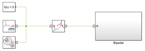
Bipedal is considered a double inverted pendulum model with complaint joints. Designed a pattern generator based on Zero-Moment Point (ZMP), for dynamic balance of the bipedal robot (Figure 1). The bipedal was learning with the RL controller after learning it stores the successful and optimal cases in a lookup table for the current environment. If the same dynamic environment is there in the next run then it executes using that lookup table reducing the number of iterations of the specific joint of the leg. But the bipedal is not fully reducing the iterations as lookup table as only the optimal actions and the corresponding next state but the reward/punishment signal is calculated on the fly each time (Figure 2).
The future of the bipedal robots is like an emotional, physical companion of human who can help humans in household chores, in a hazardous environment, as a companion and friend at the workplace.
Figure 1. ZMP Position of a Biped Walking Sequence
Figure 2. RL Model of Bipedal Robot
The proposed model considers the lower body parts of the bipedal robot. The model consists of ten degrees of freedom with each leg having five degrees of freedom. Both ends of the legs are connected to the torso. The torso is a rigid body on which both hip joints are attached and have a vision system. A Simulink/SimSpace Multibody Matlab model is designed for the bipedal. For designing and developing the lower body of bipedal, the anatomy of the human lower limb is taken into consideration. (Table 1 and 2) [6, 7]. The lower body system of the bipedal robot consists of the left leg, right leg, and torso without considering the upper body parts like shoulder, hand, and head [8, 9]. The proposed work considers the mechanical design parameters of Table 1 and Table 2 for the bipedal robot designing.
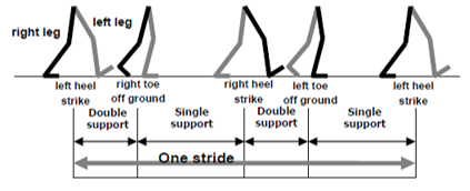
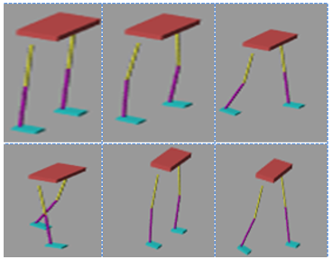
In one walking cycle (Figure 1 and Figure 3), different walking stages are present - the first stage, when both feet are on ground bipedal is stable in this position (Double Support Phase (DSP)), the second stage, when the right leg is to be lifted from the ground zero moment point (ZMP) shifts towards the toe of the right leg (DSP), third stage, the right leg swings in air ZMP is now dependent on only left leg as at this stage only one leg is on the ground and so called single support phase (SSP) and balancing is also a critical task.
Table 1. Lower body parameter
|
Parameters |
Dimension in mm |
|
Foot length |
240 |
|
Foot width |
90 |
|
Foot height |
100 |
|
Lower leg height |
380 |
|
Lower leg diameter |
370 |
|
Upper leg height |
380 |
|
Upper leg diameter |
480 |
|
Torso length |
330 |
|
Torso width |
150 |
Figure 3. Walking cycle
Fourth stage, the next stage right heel touches the ground now again ZMP is also on the right leg and DSP stage exist, the fifth stage, both the feet are on the ground and bipedal is stable. Second, third and fourth stages have stability and balancing problems which are critical in bipedal walk and have to be maintained online during the walk cycle.
The starting/initial values considered for the bipedal for the first run is ankle joint is at 0°, knee joint is at -25°, and hip join is at -15° to hip joint of the right leg and opposite values for the left leg. When gyroscope sense these values, the robot walks to the goal point. The goal point for ankle joint, knee joint, and hip joint are 20°, 20°, and 15° respectively. The legs of the bipedal robot are at some position at run time, the RL controller has a goal point to reach in along with runtime parameters which adds to stability is pelvis swing amplitude controller, damping controller, ZMP compensator, and landing orientation controller.
Even after designing the bipedal stability and smooth trajectories, online strategies (Table 3) are required for the stable landing of the foot on the ground and avoid sudden jerks while walking which will harm the bipedal [10-13].
Table 2. Joint range degree of freedom and motion
|
Joint |
Standard Human Leg (in degree) |
Proposed Humanoid leg (in degree) |
|
|
Torso |
Pitch |
-15to 130 |
-15 to 100 |
|
|
Yaw |
-45 to 50 |
-45 to 45 |
|
|
Roll |
-30 to 45 |
0 to 40 |
|
Knee |
Pitch |
-10 to 150 |
0 to 100 |
|
Ankle |
Pitch |
-20 to 50 |
-20 to 30 |
Table 3. Summary of walking algorithm
|
Control Parameters |
Real-Time Parameters |
Aim fulfilled |
|
Balance Controller |
Damping parameters (Stages 1, 3, SSPs of 2, 4) |
Reducing oscillations in the upper body in SSP (ankle joints are imposed by damping) |
|
ZMP compensator parameters (Stages 1,3, SSPs of 2, 4) |
Maintaining balance dynamically by horizontal movement of the pelvis |
|
|
Walking Pattern Control |
Pelvis swing amplitude controller (Stages DSPs of 2, 4) |
The amplitude of ZMP is considered to compensate lateral swing amplitude of pelvis |
|
Motion Control |
Landing position parameters (Stages 2, 4) |
Compensate landing position to prevent unstable landing |
The force/ torque sensor at ankle results in sustained oscillations in SSP which is overcome by damping oscillator parameters. Bipedal is a model of IP with a compliant joint.
Equation of motion is given by:
$T=m g l \theta-m l^{2} \ddot{\theta}=K(\Theta-u)$ (1)
where, u - reference joint angle, θ - actual joint angle due to compliance.
Damping control law states:
$u_{c}=u-k_{d} \widehat{\dot{\theta}}$ (2)
where, u - reference joint angle, kd - damping control gain, and uc - joint angle compensation.
According to ZMP dynamics, ZMP compensator parameters stabilize ZMP. Torso moves back and forth and side by side. Both torso movement and ZMP are controlled by the following equation
$Y_{z m p}=Y_{p e l v i s}-\frac{l}{g} \ddot{Y}_{p e l v i s}$ (3)
where, Ypelvis - lateral displacement of pelvis and YZMP - lateral ZMP.
The landing orientation controller, for comfortable landing, coordinates torque estimated after some time and stable contact by adjusting ankle joints to ground.
Landing orientation control law is given as follows:
$u_{c}=u+\frac{T(s)}{C_{L} s+K_{L}}$ (4)
where, CL - damping coefficient, KL - stiffness, u - reference angle of ankle and uc - reference ankle angle (compensated).
The landing timing controller helps in achieving stable walking gait of the bipedal by updating the walking pattern schedule during landing. This prevents the biped from falling and walking unstably in the dynamic environment. The time scheduler pauses the motion if the foot does not land on the ground, the bipedal sole is not in contact with the ground.
2.1 Simulink model of bipedal
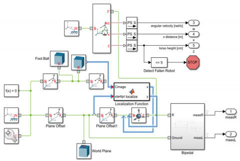
While creating the different parts of the bipedal robot, plane consideration had been taken. The torso and the hip joints are created in the frontal plane of the sketch command. The rest of the part created in the sagittal plane of the sketch (Figure 4). Torso also contains the camera mounted on it for object identification and the vision-based navigation (Figure 5 and Figure 6) [14].
In the proposed work the bipedal identifies the object and walks towards the object trying not to fall, have jerks and stop near the identified object.
Figure 4. Simulink model of bipedal robot
Figure 5. Simulink model of Bipedal with object localization and navigation in a dynamic environment
Figure 6. In explorer Simulink model of Bipedal
2.2 Forgetting mechanism incorporated in traditional Q-learning
The RL agent sometimes attempts to reuse previously learned knowledge in the dynamic environment. This knowledge may be outdated as the environment is dynamic and uncertain. This changes the exploration and exploitation dilemma. To restrict the use of previously learned knowledge which may be outdated due to change in dynamics of environment a forgetting mechanism is incorporated in the Q-learning algorithm.
In a dynamic environment, the dynamic reward and the optimal action are calculated at the run time, which accounts for the total cost associated with being in a given state. The optimal Q-values, along with the state to be selected are initialized to zero in the learning and execution phase. As RL agent first learns by exploration and after some steps, it evaluates a tradeoff between the exploitations of new states, action pair, and exploitation of choosing actions which have previously resulted in near-optimal/optimal policy. The Q-value function is a two-dimensional lookup table that is updated after each time a state is visited [15, 16]. The action selection depends on the generation of a random number. The exploitation takes place when the value of random number lies between (0, ε*ε-decay), select the greedy action and exploration when it lies between (ε*ε-decay, 1), selection of new action is done. Bipedal is trained not to get stuck at any joint while learning and executing. The large value of ε shows dependency on the subsequent following state whereas small value shows dependency on reward function. If ε →1 little forgetting takes place (behaves like traditional Q- learning algorithm). If ε→ 0 almost all rewards are forgotten between episodes (leads to an exploration of the environment).
Reward/Penalty given to RL agent depends on the distance between the current state and goal state:
reward $=e^{-\alpha(\text {Goal state of RL agent-current state of } R L \text { agent })}$ (5)
Q-learning Algorithm after incorporating the randomness:
$\begin{aligned} Q(s, a) \leftarrow Q(s, a) & \\ &+\alpha[r\\ &\left.+\gamma \max _{\mathrm{a}}, Q\left(s^{\prime}, a^{\prime}\right)-Q(s, a)\right] \end{aligned}$ (6)
The RL Algorithm for Incorporating Forgetting Mechanism proposed is as follows:
(1) The environmental parameters are decided: epsilon(ε), learning rate(α), epsilon decay, discount factor(λ)
(2) Q matrix is initialized to zero
(3) For every run -
A. Selection of Initial state is conducted (initially received by sensors, at runtime evaluated by an algorithm)
B. Do while target state has not been reached
(4) Store values of each episode and the number of iterations required to reach the target state along with the total duration for each process in the third excel file.
(5) Plot graphs for comparison of the number of iterations in the learning and execution phase along with total time for execution in each episode, total reward awarded in each episode, mean random value generated in each episode.
2.3 Reinforcement learning controller
Kinematics and dynamics analysis give real-time information to the controller of the bipedal [17, 18]. In the reinforcement control algorithm [19, 20], if the magnitude of action is too small or too large, excess time is taken to go to the next state from the current state then programmed not to stick at a specific position for more than 10 second as it affects the stability of the bipedal. RL agents are programmed by rewards. After observing the current state, the reinforcement controller is choosing an action from the available set of finite actions. After choosing an action, the corresponding leg joint moves to the next stable state. This iteration continues until the goal/target point reached by the individual joints of the bipedal. This work also considers the fall of bipedal in forward and reverse directions. Currently, the reinforcement algorithm is developed for the hip, knee, and ankle of bipedal of each leg taking into consideration contact forces of the ground.
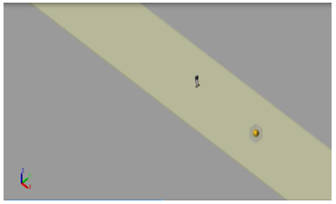
The bipedal robot decides on its own just by having information about the present state and switches to the next state without knowing the kinematics and dynamics of the system (Figure 7).
Figure 7. Locomotion of bipedal robot
When gyroscope senses the current values, helps the bipedal to reach to the goal point. The goal point for ankle joint, knee joint, and hip joint are 20°, 20°, and 15° respectively. Time taken to reach these goal angles depends on processor capabilities and not on kinematics and dynamics calculation. The reinforcement controller (Figure 8) controls the intermediate position of the joint between the start point and the target point.
Figure 8. Simulink block diagram of RL controller
The simulation of the bipedal was carried out and while learning and execution results are stored for future study. Firstly, the bipedal was learning in which exploration was the main aim while in execution exploitation was the aim.
The algorithm is characterized by the following steps:
(1) Q (s, a) updating rule
(2) The function which evaluates action to be taken
(3) Forgetting Mechanism
(4) Randomness in reward depending on the current state of
RL agent and goal state.
The goal of the proposed work is to provide enhanced performance in a dynamic environment by utilizing exploration and exploitation which can maintain a larger set of the possible solution as compared to traditional Q-learning algorithm.
The proposed work is carried out in steps including- object identification, object localization, learning by RL controller, and execution of the controller data.
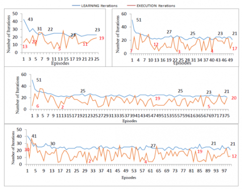
In the learning phase, bipedal is learning was tested for a different number of strides - 25, 50, 75, 100. The data obtained from learning was stored in two distinct ways: graphs and excel files/ lookup tables for future use. By comparing the strides, the data of 50, 75, and 100 showed stability in the number of iterations to learn for individual joint- hip, knee, and ankle of the bipedal.
The joints started their learning from 51 as the maximum number of iterations in those it is exploring more as compared to exploiting and reduced the learning phase iterations to 21 as a minimum which explains the optimal selection of actions and the policy to be followed by the bipedal. This in turn reduces the learning time of the bipedal too. During the learning phase, the action selection which resulted in optimal/ near-optimal policy are stored in the lookup table, which is utilized in the execution phase when bipedal come across the same situation take the data from a lookup table using exploitation.
In the execution phase, bipedal is executing from the current state for the different number of strides - 25, 50, 75, 100. The data obtained from execution was stored in two distinct ways: graphs and excel files/lookup tables for future use. By comparing the strides, the data of 50, 75, and 100 showed stability in the number of iterations to learn for individual joint- hip, knee, and ankle of the bipedal.
The maximum number of iterations in the execution phase is 18 and minimum as 2 for each joint which reveals that the bipedal is using the learned data stored in the lookup tables and the excel files. The execution is jerk-free and is smooth and seems that the bipedal is walking fast. The execution time is not reduced as the time is utilized in searching in the table the current condition and if exist then reading and using that data in execution. The number of iterations is reducing but the execution time is almost the same as the learning time. For each run of the learning and execution phase, the mean random values are evaluated by taking the mean of the random values generated in each episode of all strides. For each run of the learning and execution phase, the total rewards are evaluated by summing up the rewards generated in each episode of all strides.
The following figures reveal the above-stated points in graphical comparison.
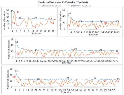
Figures 9, 10, 11 show a remarkable decrease in the number of iterations in the execution phase of the ankle, knee, and hip joint as compared to the number of iterations in the learning phase of the bipedal.
Figure 9. Comparison of Ankle for 25, 50, 75, 100 strides
Figure 10. Comparison of Knee for 25, 50, 75, 100 strides
Figure 11. Comparison of Hip for 25, 50, 75, 100 strides
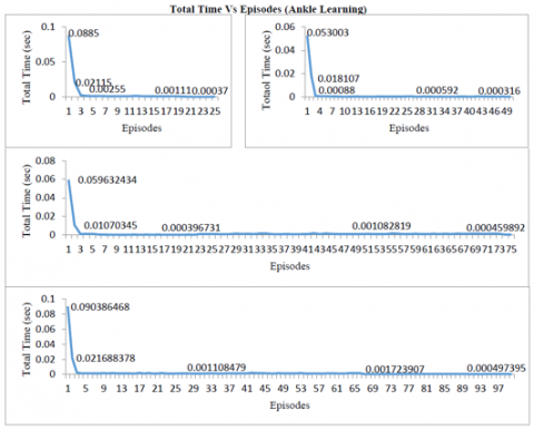
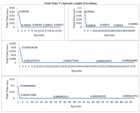
Figure 12. Comparison of ankle learning for 25, 50, 75, 100 strides
Figure 13. Comparison of ankle execution for 25, 50, 75, 100 strides
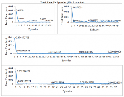
Figure 14. Comparison of hip learning for 25, 50, 75, 100 strides
Figure 15. Comparison of hip execution for 25, 50, 75, 100 strides
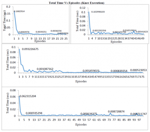
Figure 16. Comparison of knee learning for 25, 50, 75, 100 strides
Figure 17. Comparison of Knee execution for 25, 50, 75, 100 strides
Figure 12 and 13 show the total time taken by the learning and execution phase of the ankle joint. As the graph reveals the number of strides increases the curves differ because of more time required to store optimal data in the lookup table in the learning phase and for searching and reading if required data exist in the lookup table in the execution phase.
Figure 14 and 15 show the total time taken by the learning and the execution phase of the hip joint. As the graph reveals the number of strides increases the curves differ because of more time required to store optimal data in the lookup table in the learning phase and for searching and reading if required data exist in the lookup table in the execution phase. The maximum variations are in 100 stride case and some in 50 stride execution phases as compared to the learning phase.
Figure 16 and 17 show the total time taken by the learning and execution phase of the knee joint. As the graph reveals the number of strides increases the curves differ because of more time required to store optimal data in the lookup table in the learning phase and for searching and reading if required data exist in the lookup table in the execution phase. The maximum variations are in 50 strides and 100 strides. This irregular variation as compared to hip and ankle joint is due to the reason that the knee joint has maximum negative and positive values it can take (-45 to 45). The variation in the angle of the knee is maximum as compared to the hip and ankle while walking.
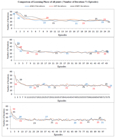
Figure 18. Comparison of the learning phase of all three joints
Figure 18 above and 19 below show the comparison of the learning phase and the execution phase of all the three joints simultaneously. In the learning phase, the variation in the three joints is more when the strides are 25 and 50 and mostly coincides when they reach 75 and 100 strides. This reveals as the stride increases the bipedal first explores the dynamic environment then after some strides start exploiting the optimal actions and policies for getting maximum rewards. The execution phase is using the lookup data which has the optimal action and policy stored but the variations are more sometimes for some abrupt cases. But for most of the cases, they are within the limit taking the minimum value to be 2 in the execution phase. These random nesses cannot be controlled in this work as the values are taken from the lookup table at the runtime which is not predefined. This shows that the reinforcement learning controller executes the step of gait by using data from the lookup table on the fly depending upon the random number of generations and the random reward generation. These values are calculated on the fly when the execution phase is in progress.
Figure 19. Comparison of the execution phase of all three joints
The reinforcement controller is implemented to switch the bipedal robot from the current state to the next state, controller trains hip joint first then the knee joint is trained then training of ankle joint is carried out.
The previous knowledge is not used to train the joints of biped as the knowledge is outdated as the environment is dynamic and uncertain. The training of biped depends on the dynamics of the system. Biped is trained and knowledge gained is used for exploration or exploitation steps which depends on the random value which is incorporated in the algorithm then after that the forgetting mechanism is also implemented by setting the value of variable large so that it forgets the old information and gains new states which depend on dynamics of the current system. The reward function is also not predefined or has constant value but it is calculated on the fly by evaluating the distance between the goal and the current state and doing some algebraic and exponential operations. The bipedal is trained not to stick in any position for more than specific iterations of the training algorithm ie should be off the struck position in few seconds and also trained not to change its value drastically so that it would harm the hardware of the bipedal system like servomotor, sensors, etc by passing too high or too low values to the individual parts and should not stop abruptly that is standing still or fall.
The bipedal has a limitation of the degree of freedom not considering the upper part (hand and shoulder joint) of the body which also plays an important role in the gait of bipedal. The execution phase is sometimes executing 18 iterations which require a considerable amount of time and show variations in the graph of rewards generation. This can be minimized more as in some cases it reached 2 iterations but not always.
[1] Sutton, R.S., Barto, A.G. (1998). Reinforcement Learning: An Introduction. MIT Press, Cambridge, MA.
[2] Watkins, C. (1989). Learning from Delayed Rewards. Ph.D. Dissertation, Cambridge University http://www.cs.rhul.ac.uk/~chrisw/new_thesis.pdf, accessed on 20 Jul. 2020.
[3] Sharma, R., Prateek, M., Sinha, A.K. (2013). Use of reinforcement learning as a challenge: A review. International Journal of Computer Application, 69(22): 28-34. https://doi.org/10.5120/12105-8332
[4] Stone, P., Veloso, M. (2000). Multiagent systems: A survey from a machine learning perspective. Autonomous Robots, 8: 345-383. https://doi.org/10.1023/A:1008942012299
[5] Whitehead, S.D. (1992). Reinforcement learning for the adaptive control of perception and action. Technical Report 406, The University of Rochester.
[6] Berns, K., Dillmann, R., Zachmann, U. (1992). Reinforcement-learning for the control of an autonomous mobile robot. Proceedings of the IEEE/RSJ International Conference on Intelligent Robots and Systems, Raleigh, NC, USA, pp. 1808-1815. https://doi.org/10.1109/IROS.1992.601414
[7] Yen, G.G., Hickey, T.W. (2004). Reinforcement learning algorithms for robotic navigation in dynamic environments. ISA Transactions, 43(2): 217-230. https://doi.org/10.1016/S0019-0578(07)60032-9
[8] Azouaoui, O., Cherifi, A., Bensalem, R., Farah, A., Achour, K. (2006). Reinforcement learning-based group navigation approach for multiple autonomous robotic systems. Advanced Robotics, 20(5): 519-542. https://doi.org/10.1163/156855306776985531
[9] Jaradat, M.A.K., Al-Rousan, M., Quadan, L. (2011). Reinforcement based mobile robot navigation in a dynamic environment. Robotics and Computer-Integrated Manufacturing, Elsevier, 27(1): 135-149. https://doi.org/10.1016/j.rcim.2010.06.019
[10] Gill, C.R., Calvo, H., Sossa, H. (2019). Learning an efficient gait cycle of a biped robot based on reinforcement learning and artificial neural networks. Applied Science, 9(3): 502. https://doi.org/10.3390/app9030502
[11] Hwang, K.S., Li, J.L., Li, J.S. (2016). Biped balance control by reinforcement learning. Journal of Information Science and Engineering, 32: 1041-1060.
[12] Raj, S., Kumar, C.S. (2013). Q learning-based reinforcement learning approach to bipedal walking control. Proceedings of the 1st International and 16th National Conference on Machines and Mechanisms (iNaCoMM2013), IIT Roorkee, India, pp. 618-620.
[13] Weiβ, G. (1995). Distributed reinforcement learning. Robotics and Autonomous Systems, 15(1-2): 135-142. https://doi.org/10.1016/0921-8890(95)00018-B
[14] Bharadwaj, D., Prateek, M., Sharma, R. (2019). Development of reinforcement control algorithm of the lower body of autonomous humanoid robot. International Journal of Recent Technology and Engineering (IJRTE), 8(1): 915-919.
[15] Sharma, R., Singh, I., Bharadwaj, D., Prateek, M. (2019). Incorporating forgetting mechanism in Q, learning algorithm for locomotion of bipedal walking robot. International Journal of Innovative Technology and Exploring Engineering (IJITEE), 8(7): 1782-1787.
[16] Sharma, R., Singh, I., Prateek, M., Pasricha, A. (2019). Implementation of feature-based object identification in bipedal walking robot. International Journal of Engineering and Advanced Technology (IJEAT), 8(5): 110-113.
[17] Maravall, D., de Lope, J., Domínguez, R. (2012). Coordination of communication in robot teams by reinforcement learning. Robotics and Autonomous Systems, 61(7): 661-666. https://doi.org/10.1016/j.robot.2012.09.016
[18] Stone, P., Sutton, R.S. (2001). Scaling reinforcement learning toward RoboCup soccer. In Proceedings the Eighteenth International Conference on Machine Learning, Williamstown, MA, USA, pp. 537-544.
[19] Duan, Y., Liu, Q., Xu, X.H. (2007). Application of reinforcement learning in robot soccer. Engineering Applications of Artificial Intelligence, 20(7): 936-950. https://doi.org/10.1016/j.engappai.2007.01.003
[20] Kumar, A., Paul, N., Omkar, S.N. (2018). Bipedal walking robot using deep deterministic policy gradient. arXiv:1807.05924v2 [cs.RO]