Xingwang Liu | Haitao Li | Bingyu Wang | Li Zhao | Jiadi Liu*
© 2020 IIETA. This article is published by IIETA and is licensed under the CC BY 4.0 license (http://creativecommons.org/licenses/by/4.0/).
OPEN ACCESS
In engineering practice, to make sure that a project can achieve safe operation while minimizing the overall cost during the whole life cycle, the supervisor of the project generally needs to make optimal decisions for the Life Cycle Cost (LCC) of the project. To this end, this paper adopted Genetic Algorithms (GA) and LCC theory to propose and implement a kind of optimization algorithms suitable for solving maintenance scheme problems. Combining with the selection of three actual maintenance scenarios of “take no maintenance measure/preventive maintenance measures only”, “take major maintenance measures”, and “take major maintenance measures and preventive maintenance measures”, the proposed algorithm adopted real number coding to give optimization solutions from two perspectives of “control service life and calculate cost” and “control cost and calculate service life”; moreover, the paper conducted a comparative analysis on the maintenance schemes of reinforced concrete bridge decks using Matlab and verified the reliability and efficiency of the proposed algorithm.
life cycle cost (LCC), intelligent optimization, genetic algorithm (GA), optimal solution, maintenance scheme
At present, a large number of highway and bridge projects in China are suffering from structural defects and structural aging problems, urgently need to be repaired, strengthened, reconstructed, or even demolished and rebuilt. However, a country’s financial resources are often limited, so it is necessary for us to reasonably allocate and make good use of the funds, and adopt appropriate solutions at the right time, so as to achieve the goal of saving the cost to the greatest extent. For a long time, a lot of researches have been done at home and abroad on bridge structure optimization schemes and the economy of the corresponding maintenance schemes. The theory of Life Cycle Cost (LCC) was first applied to procurement of expensive military equipment in the United States and then introduced to the field of engineering, its purpose is to manage the decision-making at various stages in the life cycle of engineering projects. The US Federal Highway Administration (FHWA) was the first to introduce the application of LCC theory in bridge engineering [1]. Then Hawk proposed a LCC analysis method suitable for bridge structures [2]; and Scott et al. conducted an in-depth study on decision-making and economic analysis of bridge decks [3-5]. At present, commonly-used optimization methods include mathematical planning methods and artificial intelligence optimization methods, wherein the mathematical planning methods generally have the characteristics of unstable solution and slow operation speed [6], and the artificial intelligence optimization methods include Genetic Algorithm (GA), Particle Swarm Optimization (PSO), and Artificial Bee Colony (ABC) algorithm, etc. [7-8]. Holland first applied GA to the optimization and selection of plans, and then GA has become a typical heuristic random search algorithm [9-11]. He Hongming used Neural Network (NN) to study the evaluation, prediction and maintenance decision of the deterioration of existing reinforced concrete structures [12-15]. Based on the specified service level, Liu Xingwang adopted GA as the tool to optimize the pavement maintenance decision-making scheme, and introduced LCC theory and GA to the optimization of the maintenance scheme of the bridge decks [16-18].
From the comparison of previous studies, we can know that, how to establish suitable models for specific engineering problems and improve the efficiency and accuracy of calculation are the key issues that need to be solved at present. Due to its parallel and global optimization characteristics, GA is more suitable for optimizing decisions. Based on the LCC theory, with MATLAB as the development platform, this paper combines with GA to compile algorithm that is suitable for the cost optimization of the maintenance schemes for reinforced concrete bridge decks, and verifies the reliability and efficiency of the proposed algorithm with actual examples.
2.1 Description of the problem
LCC analysis is the basis of engineering projects and scheme optimization, this paper took the reinforced concrete bridge deck as the research object, the initial reliability was set to be β=8.0, the degradation start time was set as T1=15, and the minimum reliability index was β*=4.2. Considering the optimization calculation of LCC, three basic maintenance scenarios were set up through GA, respectively are: take no maintenance measure/preventive maintenance measures only, take major maintenance measures, and take major maintenance measures and preventive maintenance measures. The expected target and output were the optimal cost and service life under the constraints of the three scenarios.
The calculation formula for the LCC of the example engineering project over the entire life cycle [16] is as follows:
$L C C(T)=C_{c}+C_{I N}(T)+C_{M}(T)+C_{R}(T)+C_{F}(T)$ (1)
where, Cc is the initial cost; CIN(T) is the test cost; CM(T) is the routine maintenance cost; CR(T) is the maintenance cost and the loss cost caused by the maintenance; CF(T) is the failure cost, namely the loss caused by failure.
2.2 Determination of parameters
2.2.1 Initial cost Cc
Since the initial cost won’t affect the choice of scheme, to simplify the process of comparative analysis, Cc was set to be a constant.
2.2.2 Routine test maintenance cost CIN,M(t)
To facilitate computation, the routine test cost CIN(T) and the routine maintenance cost CM(T) are generally combined together as the routine test & maintenance cost CIN,M(t), which is calculated in years.
$C_{I N, M}(t)=0.02(1+0.05 t) C_{c},\left(t<T_{1}\right)$ (2)
$C_{I N, M}(t)=0.02\left[1+0.05 t+0.5 \frac{\left[\alpha_{1}+\alpha^{'}\left(t-T_{1}\right)\right]\left(t-T_{1}\right)^{0.8}}{\beta^{*}}\right] C_{c},\left(t \geq T_{1}\right)$ (3)
where, T1 is the start time of initial degradation, its value took 15 in this paper; α1is the degradation rate at the start time of initial degradation, its value took 0.01 in this paper; α' is the increase coefficient of the degradation rate, it’s a variate [16].
2.2.3 Maintenance cost
According to LCC theory, the maintenance cost is divided into two parts, namely the preventive maintenance cost CR,PM and the reinforcement maintenance cost CR,EM. Considering the actual situation of the example, the two parts of the maintenance cost are:
$C_{R, P M}=0.1 C_{C}+C_{C} \times\left(\frac{\Delta A}{0.05}\right)^{2}$ (4)
$C_{R, E M}=C_{R, E M}(\Delta \beta)$ (5)
where, $\Delta A$ is the difference in the degradation rate before and after the maintenance; $\Delta \beta$ is the difference in the reliability index before and after the maintenance.
2.2.4 Structural failure loss CF(t)
Structural failure loss is usually related to the failure level, the classification method of failure level adopted in this paper is shown in Table 1, and the corresponding calculation formula for failure loss is shown as Formula 7.
Table 1. Reliability indexes of failure levels
|
Structural failure level di |
Intact (i=1) |
Slight (i=2) |
Medium (i=3) |
Serious (i=3) |
Very serious (i=5) |
|
Reliability index |
β-2.0 |
β-1.5 |
β-1.0 |
β-0.5 |
β |
|
Direct loss coefficient kCF1 |
0.01 |
0.20 |
0.50 |
1.0 |
2.0 |
|
Ratio of direct loss to indirect loss kF |
0.1 |
0.5 |
5.0 |
50.0 |
500.0 |
Structural failure loss CF(t) can be calculated as follows:
$C_{F}(t)=\sum_{i=1}^{5}\left\{p_{f}^{i}(t) \times C_{c} \times k^{i}_{C F 1}\left(1+k_{F}^{i}\right)\right\}$ (6)
where, $p_{f}^{i}(t)$ is the failure probability of the structure, and its calculation formula [16] is:
$p_{f}=\frac{1}{2}\left(1+\alpha_{1} \beta+\alpha_{2} \beta^{2}+\alpha_{3} \beta^{3}+\alpha_{4} \beta^{4}+\alpha_{5} \beta^{5}+\alpha_{6} \beta^{6}\right)^{-16}$ (7)
where,
α1=0.049867374; α2=0.0211410061; α3=0.0032776263;
α4=0.00003800036; α5=0.0000488906; α6=0.000005383.
2.2.5 The overall objective of the example project
The overall objective of the example project took account both economy and safety issues, that is, achieve maximum expected service life while the structure satisfies the constrain of safe operation; or achieve minimum expected project cost under the condition that the benefits of the project can hardly be estimated accurately.
The overall objective of the example project can be expressed as:
$\operatorname{Max}\{E[U(T)]-E[L C C(T)]\}$ or $\operatorname{Min} E[L C C(T)]$ (8)
subject to $\beta \geq \beta^{*}$ or $p_{s} \geq p_{s}^{*}$ (9)
where, $E[U(T)]$ is the sum of expected benefits within the life cycle $(T)$ of the project; $\beta$ is the structural reliability index (within service life); $\beta^{*}$ is the limit of target reliability index (the lowest target reliability index during the trial period); $p_{s}$ is the structural reliability (within service life); $p_{s}^{*}$ is the limit of target reliability (the lowest target reliability during the trial period)
In this paper, the overall objective of the example project was set as a constraint for the optimization of the scheme. The scheme optimization was conducted from two aspects of “satisfying a certain service life and calculating the minimum cost” and “satisfying a certain cost and calculating the longest service life”.
3.1 Individual coding
This paper adopted real number coding [19-22], each gene was represented by a character set and composed of I (number of maintenance measures) strings (sub-genes), as shown in Figure 1, J1 represents the set of reinforcement measures, the numbers 1-6 represent the reinforcement measures, as shown in Formula 10; J2 represents the set of maintenance measures, the numbers 1-4 represent the maintenance measures, as shown in Formula 11.
Figure 1. Gene coding
$J_{1}=\left\{\begin{array}{l}1-\text { Reinforce in the } 30^{t h} \text { year } \\ 2-\text { Reinforce in the } 40^{t h} \text { year } \\ 3-\text { Reinforce in the } 50^{t h} \text { year } \\ 4-\text { Reinforce in the } 60^{t h} \text { year } \\ 5-\text { Reinforce in the } 70^{t h} \text { year } \\ 6-\text { No reinforcement }\end{array}\right.$ (10)
$J_{2}=\left\{\begin{array}{l}1-\text { No maintenance } \\ 2 \text { - Maintain every } 10 \text { years } \\ 3 \text { - Maintain every } 20 \text { years } \\ 4-\text { Maintain every } 30 \text { years }\end{array}\right.$ (11)
3.2 Population initialization
Generally, the individuals in the initial population are generated randomly, because without prior knowledge of the problem space, it is difficult to judge the number of optimal solutions and their distribution in the feasible solution space. This paper adopted the method of randomly generated initial population, that is, for the first part (J1) of each individual, a random number between 1-6 was generated by the randi (6) function; for the second part (J2) of each individual, a random number between 1-4 was generated by the randi (4) function; at last, the initial population (pop) was formed by multiple random individuals, and the initial population was a two-dimensional matrix.
3.3 Individual assessment
In this paper, the individual fitness function was consistent with the optimization goal. The individual fitness value was calculated by Formula (1), and ensured to satisfy the constraint condition Formula (9); individuals that did not satisfy the constraint were not allowed to enter the selection stage.
3.4 Selection, crossover, and mutation operations
This paper adopted Roulette Wheel Selection as the selection method [23-26]. Individuals with high fitness values (low LCC value) have a higher probability of being selected, while individuals with low fitness values (high LCC value) have a higher probability of being eliminated.
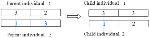
In this paper, the crossover operation adopted the single-point crossover scheme according to the particularity of the model. That is, from that population that had been subject to the selection operation, two individuals were chosen as the objects for the crossover operation, and these two individuals are called the parent individuals, which were subject to single-point crossover operation and two new individuals were generated, and called the child individuals, as shown in Figure 2. From J1 or J2, a position was randomly selected as the intersection point, which was taken as the position of the first gene of the gene string of parent individual 1 and parent individual 2; then the gene codes after the intersection point were interchanged to form the child individual 1 and child individual 2, the crossover operations of other individuals were completed in the same way.
Figure 2. Crossover operation
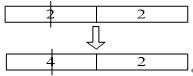
In this paper, the mutation operation adopted the substitution mutation-based scheme, that is, a position was randomly selected for substitution, and the genetic information used for substitution was made sure to be the one that can satisfy the reinforcement maintenance measures, as shown in Figure 3.
Figure 3. Mutation operation
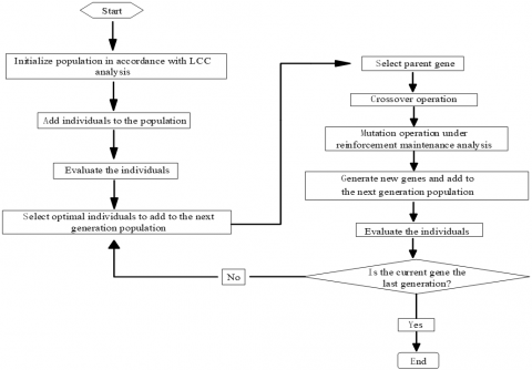
3.5 Algorithm implementation
After trials and loops, the algorithm finally obtained the minimum value of the objective function as shown in Figure 4.
Figure 4. Flow of GA
According to the engineering project example in [16] we can know that, under the condition of no maintenance measure had been applied, the service life of concrete bridge deck is 70 years. From two perspectives, this paper set three different maintenance scenarios and conducted comparative analysis from the vertical and horizontal directions, as shown in Table 2. With MATLAB R2013a software as the operating platform, LCC theory as the basis, Formula (1) as the objective function, the overall objective of the example project as the constraint condition, a GA program was written and compiled to optimize the schemes that satisfied the conditions and find out the optimal solution. The parameters of the evolutionary algorithm are shown in the schemes listed in sections 3.1 to 3.3.
Table 2. Reliability indexes of failure levels
|
|
Perspective 1: control the service life, and calculate the cost |
Perspective 2: control the cost and calculate the service life |
|
Scenario 1 |
A No maintenance |
|
|
B Maintain every 10 years |
||
|
C Maintain every 20 years |
||
|
D Maintain every 30 years |
||
|
Scenario 2 |
A Reinforce in the 30th year |
|
|
B Reinforce in the 40th year |
||
|
C Reinforce in the 50th year |
||
|
D Reinforce in the 60th year |
||
|
E Reinforce in the 70th year |
||
|
Scenario 3 |
A Reinforce in the 30th year and maintain every 10, 20, and 30 years |
|
|
B Reinforce in the 40th year and maintain every 10, 20, and 30 years |
||
|
C Reinforce in the 50th year and maintain every 10, 20, and 30 years |
||
|
D Reinforce in the 60th year and maintain every 10, 20, and 30 years |
||
|
E Reinforce in the 70th year and maintain every 10, 20, and 30 years |
||
4.1 Optimal scheme for no maintenance measure and preventive maintenance measures only
4.1.1 Control the service life and calculate the cost
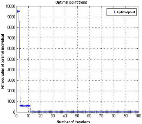
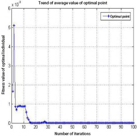
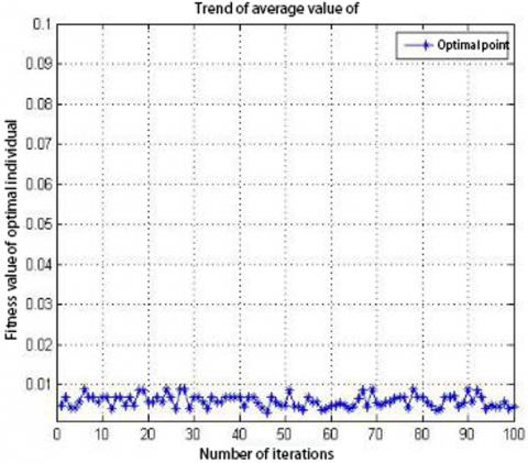
Figure 5. Trend of optimal point
Figure 6. Trend of average value of optimal point
The optimization goal is to calculate the scheme with the minimum cost under the constraint condition that the service life is 100 years. In terms of Scenario 1, the evolution parameters were set as follows: population size 100, number of iterations 100 generations, crossover rate 0.4, mutation rate 0.1. Targeting at the optimization goal, the maintenance scheme was optimized by the GA program, and the data results and analysis are shown as follows:
(1) Calculation results:
After the optimization operations, the specific cost and optimization process of each maintenance scheme are shown in Table 3, and the convergence diagrams are shown in Figure 5 and Figure 6
(2) Result analysis
Table 3 shows the optimization process of the schemes under Scenario 1 by GA, the total cost of the initial scheme was 9.50E + 03CC, and the scheme was “no measure taken”; after the optimization operation, it reached optimum in the 13th generation and converged to the end; the total cost after optimization was 7.856CC, and the scheme was “maintain every 10 years”. Figure 5 shows the trend of the individual with the optimal fitness value and Figure 6 shows the trend of the average fitness value of the optimal solution. It can be seen that the algorithm had good convergence characteristics and high solution efficiency. The calculation results were compared with the existing examples [16], and its rationality had been proved. Since the GA had found the optimal solution quickly and accurately, its high efficiency had been proved as well.
Table 3. Data summary of schemes
|
Number of iterations |
Schemes |
$C_{IN,M}$ |
$C_{F}$ |
$C_{R, P M}$ |
$L C C$ |
|
1 |
No measure taken |
7.6355 $C_{c}$ |
9.50E+03 $C_{c}$ |
0.2 $C_{c}$ |
9.50E+03 $C_{c}$ |
|
2 |
No measure taken |
7.6355 $C_{c}$ |
9.50E+03 $C_{c}$ |
0.2 $C_{c}$ |
9.50E+03 $C_{c}$ |
|
3 |
Maintain every 30 years |
7.6355 $C_{c}$ |
591.3107 $C_{c}$ |
0.2001 $C_{c}$ |
599.1463 $C_{c}$ |
|
4 |
Maintain every 30 years |
7.6355 $C_{c}$ |
591.3107 $C_{c}$ |
0.2001 $C_{c}$ |
599.1463 $C_{c}$ |
|
… |
… |
… |
… |
… |
… |
|
13 |
Maintain every 10 years |
7.6355 $C_{c}$ |
0.0196 $C_{c}$ |
0.2009 $C_{c}$ |
7.856 $C_{c}$ |
|
… |
… |
… |
… |
… |
… |
|
100 |
Maintain every 10 years |
7.6355 $C_{c}$ |
0.0196 $C_{c}$ |
0.2009 $C_{c}$ |
7.856 $C_{c}$ |
4.1.2 Control the cost and calculate the service life
The optimization goal is to calculate the scheme with the longest service life under the constraint condition of a given total maintenance cost. In this paper, the initial cost Cc was set to 1 million yuan, the limit of total maintenance cost was set to 7 million yuan, and the constraint condition was Formula (9). According to the reliability degradation model [16] and Formula (1), a GA optimization program was written and compiled using MATLAB to calculate the service life under the Scenario 1.
(1) Calculation results:
Table 4 Service life of maintenance schemes
|
Number |
Scheme |
Service life |
Reliability |
|
1 |
Routine maintenance |
77 |
3.5188 |
|
2 |
Maintain every 10 years |
93 |
5.1282 |
|
3 |
Maintain every 20 years |
91 |
4.0322 |
|
4 |
Maintain every 30 years |
84 |
3.6213 |
(2) Result analysis
According to the results in Table 4, it can be seen that the service life was the longest 93 years when the scheme was “maintain every 10 years”, and the corresponding reliability value was 5.1282. It can be seen from the results that the shorter the interval, the longer the service life extended, this result is consistent with the existing research conclusions [16], which proved the rationality of the algorithm.
4.2 Optimal scheme for major maintenance measures
4.2.1 Control the service life and calculate the cost
The optimization goal is to calculate the scheme with the minimum cost under the constraint condition that the service life is 100 years. In terms of Scenario 2, the evolution parameters were set as follows: population size 100, number of iterations 100 generations, crossover rate 0.4, mutation rate 0.1. Targeting at the optimization goal, the maintenance scheme was optimized by the GA program, and the data results and analysis are shown as follows:
(1) Calculation results:
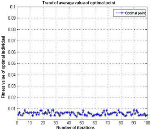
After the optimization operations, the specific cost and optimization process of each maintenance scheme are shown in Table 5, and the convergence diagrams are shown in Figure 7 and Figure 8.
Figure 7. Trend of optimal point
Figure 8. Trend of average value of optimal point
(2) Result analysis
Table 5. Data summary of schemes
|
Number of iterations |
Scheme |
$C_{IN,M}$ |
$C_{F}$ |
$C_{R, P M}$ |
$L C C$ |
|
1 |
Reinforce in the 70th year |
7.6355 $C_{c}$ |
0.4759 $C_{c}$ |
0.4329 $C_{c}$ |
8.5443 $C_{c}$ |
|
2 |
Reinforce in the 60th year |
7.6355 $C_{c}$ |
0.0198 $C_{c}$ |
0.5589 $C_{c}$ |
8.2142 $C_{c}$ |
|
3 |
Reinforce in the 60th year |
7.6355 $C_{c}$ |
0.0198 $C_{c}$ |
0.5589 $C_{c}$ |
8.2142 $C_{c}$ |
|
… |
… |
… |
… |
… |
… |
|
6 |
Reinforce in the 50th year |
7.6355 $C_{c}$ |
0.0294 $C_{c}$ |
0.4329 $C_{c}$ |
8.0978 $C_{c}$ |
|
… |
… |
… |
… |
… |
… |
|
100 |
Reinforce in the 50th year |
7.6355 $C_{c}$ |
0.0294 $C_{c}$ |
0.4329 $C_{c}$ |
8.0978 $C_{c}$ |
Table 5 shows the optimization process of the schemes under Scenario 2 by GA, the total cost of the initial scheme was 8.5443CC, and the scheme was “reinforce in the 70th year”; after optimization operation, it reached optimum in the 6th generation and converged to the end; after optimization, the total cost was 8.0978CC, and the scheme was “reinforce in the 50th year”. Figure 7 shows the trend of the individual with the optimal fitness value and Figure 8 shows the trend of the average fitness value of the optimal solution. The results showed that, under the constraint of 100-year service life, the cost of the “reinforce in the 50th year” scheme was the lowest.
4.2.2 Control cost and calculate the service life
The initial cost Cc was set to 1 million yuan, the limit of total maintenance cost was set to 7 million yuan, and the constraint condition was Formula (9). According to the reliability degradation model and Formula (1), a GA optimization program was written and compiled using MATLAB to calculate the service life of the schemes under Scenario 2.
(1) Calculation results
The Calculation results is as shown in table 6.
(2) Result analysis
According to the results in Table 6, it can be seen that the service life reached the longest 59 years when the scheme was “reinforce in the 70th year”, and the corresponding reliability value was 5.5229. From the degradation curve of reliability, we can know that, the longer the service life, for the same interval, the greater the difference of in reliability ($\Delta \beta$), and the longer the extended service life ($\Delta T$) after the reinforcement.
Table 6. Service life of maintenance schemes
|
Number |
Scheme |
Service life |
Reliability |
|
1 |
Reinforce in the 30th year |
19 |
7.9394 |
|
2 |
Reinforce in the 40th year |
29 |
7.6284 |
|
3 |
Reinforce in the 50th year |
39 |
7.1103 |
|
4 |
Reinforce in the 60th year |
49 |
6.4045 |
|
5 |
Reinforce in the 70th year |
59 |
5.5229 |
4.3 Optimal scheme for major maintenance measures and preventive maintenance measures
4.3.1 Control the service life and calculate the cost
The optimization goal is to calculate the scheme with the minimum cost under the constraint condition that the service life is 100 years. In terms of Scenario 3, under the condition of reinforcement only, the evolution parameters were set as follows: population size 100, number of iterations 100 generations, crossover rate 0.4, mutation rate 0.1. Targeting at the optimization goal, the maintenance schemes were optimized by the GA program, and the data results and analysis are shown as follows:
(1) Calculation results:
After the optimization operations, the specific cost and optimization process of each maintenance scheme are shown in Table 7, and the convergence diagrams are shown in Figure 9 and Figure 10.
Table 7. Data summary of schemes
|
Number of iterations |
Scheme |
$C_{IN,M}$ |
$C_{F}$ |
$C_{R, P M}$ |
$L C C$ |
|
1 |
Reinforce in the 70th year and conduct routine maintenance afterwards |
7.6355 $C_{c}$ |
0.3990 $C_{c}$ |
0.7043 $C_{c}$ |
8.7388 $C_{c}$ |
|
2 |
Reinforce in the 50th year and conduct routine maintenance afterwards |
7.6355 $C_{c}$ |
0.0294 $C_{c}$ |
0.4329 $C_{c}$ |
8.0978 $C_{c}$ |
|
3 |
Reinforce in the 50th year and conduct routine maintenance afterwards |
7.6355 $C_{c}$ |
0.0294 $C_{c}$ |
0.4329 $C_{c}$ |
8.0978 $C_{c}$ |
|
… |
… |
… |
… |
… |
… |
|
6 |
Maintain every 10 years |
7.6355 $C_{c}$ |
0.0196 $C_{c}$ |
0.2009 $C_{c}$ |
7.8560 $C_{c}$ |
|
… |
… |
… |
… |
… |
… |
|
100 |
Maintain every 10 years |
7.6355 $C_{c}$ |
0.0196 $C_{c}$ |
0.2009 $C_{c}$ |
7.8560 $C_{c}$ |
Figure 9. Trend of optimal point
Figure 10. Trend of average value of optimal point
(2) Result analysis
Table 7 shows the optimization process of schemes under Scenario 3 by GA, the total cost of the initial scheme was 8.7388CC, and the scheme was “reinforce in the 70th year and conduct no maintenance afterwards”; after optimization operation, it reached optimum in the 6th generation and converged to the end; the total cost after optimization was 7.8560CC, and the scheme was “maintain every 10 years”. Figure 9 shows the trend of the individual with the optimal fitness value and Figure 10 shows the trend of the average fitness value of the optimal solution. The results showed that, among the schemes for major maintenance measures and preventive maintenance measures, the optimal scheme that satisfied the constraint was “maintain every 10 years”.
4.3.2 Control cost and calculate the service life
The initial cost Cc was set to 1 million yuan, the limit of total maintenance cost was set to 7 million yuan, and the constraint condition was Formula (9). According to the reliability degradation model and Formula (1), a GA optimization program was written and compiled using MATLAB to calculate the service life of the schemes under Scenario 3.
(1) Calculation results:
Table 8. Service life of maintenance schemes
|
Number |
Scheme |
Service life |
Reliability |
|
1 |
Maintain every 10 years |
93 |
5.1282 |
|
2 |
Reinforce in the 30th year and maintain every 10 years afterwards |
19 |
7.9394 |
|
3 |
Reinforce in the 30th year and maintain every 20 years afterwards |
19 |
7.9394 |
|
4 |
Reinforce in the 30th year and maintain every 30 years afterwards |
19 |
7.9394 |
|
5 |
Reinforce in the 40th year and maintain every 10 years afterwards |
29 |
7.6284 |
|
6 |
Reinforce in the 40th year and maintain every 20 years afterwards |
29 |
7.6284 |
|
7 |
Reinforce in the 40th year and maintain every 30 years afterwards |
28 |
7.6692 |
|
8 |
Reinforce in the 50th year and maintain every 10 years afterwards |
39 |
7.1103 |
|
9 |
Reinforce in the 50th year and maintain every 20 years afterwards |
38 |
7.1707 |
|
10 |
Reinforce in the 50th year and maintain every 30 years afterwards |
38 |
7.1707 |
|
11 |
Reinforce in the 60th year and maintain every 10 years afterwards |
49 |
6.4045 |
|
12 |
Reinforce in the 60th year and maintain every 20 years afterwards |
49 |
6.4045 |
|
13 |
Reinforce in the 60th year and maintain every 30 years afterwards |
49 |
6.4045 |
|
14 |
Reinforce in the 70th year |
59 |
5.5229 |
|
15 |
Reinforce in the 70th year and maintain every 10 years afterwards |
59 |
5.5229 |
|
16 |
Reinforce in the 70th year and maintain every 20 years afterwards |
59 |
5.5229 |
|
17 |
Reinforce in the 70th year and maintain every 30 years afterwards |
59 |
5.5229 |
(2) Result analysis
Under the conditions of initial cost Cc was 1 million yuan, the limit of total maintenance cost was 7 million yuan, and the constraint was Formula (9), according to the results in Table 8, it can be seen that the service life reached the longest 93 years when the scheme was “maintain every 10 years”, and the corresponding reliability value was 5.1282, indicating that among the maintenance schemes that satisfied the constraint, under condition of a given cost, the service life of the scheme “maintain every 10 years” was the longest. This result corresponded to the results in Table 7, which proved the excellency of the scheme and the rationality of the result.
Based on the LCC model, this paper studied the optimization selection problem of the maintenance schemes of reinforced concrete bridge decks. The paper used GA to design an algorithm which adopted real number coding and combined with the selection of actual maintenance schemes to optimize and analyze the cost and service life of bridge deck under the three scenarios of “take no maintenance measure/preventive maintenance measures only”, “take major maintenance measures”, and “take major maintenance measures and preventive maintenance measures”; moreover, from the two perspective of “control service life and calculate the cost” and “control the cost and calculate the service life”, the paper optimized and solved the corresponding optimal schemes, and verified the reliability and efficiency of the proposed algorithm with actual examples.
The study was supported by the Science Foundation of the Department of Education of Hebei Province (No. ZD2019117), the Science Foundation of the Hebei Provincial Department of water resources (No. 2019-49), the Science Foundation of the Hebei Agricultural University (No. LG201803), and the Science Foundation of the Hebei Agricultural University (No. bhxt201826).
[1] Gheibi, M., Karrabi, M., Shakerian, M., Mirahmadi, M. (2018). Life cycle assessment of concrete production with a focus on air pollutants and the desired risk parameters using genetic algorithm. Journal of Environmental Health Science and Engineering, 16(1): 89-98. https://doi.org/10.1007/s40201-018-0302-x
[2] Jang, B., Mohammadi, J. (2019). Impact of fatigue damage from overloads on bridge life-cycle cost analysis. Bridge Structures, 15(4): 181-186. https://doi.org/10.3233/BRS-190153
[3] Rehman, S.K.U., Ibrahim, Z., Memon, S.A., Jameel, M. (2016). Nondestructive test methods for concrete bridges: A review. Construction and building materials, 107: 58-86. https://doi.org/10.1016/j.conbuildmat.2015.12.011
[4] Fiorillo, G., Ghosn, M. (2019). Risk-based importance factors for bridge networks under highway traffic loads. Structure and Infrastructure Engineering, 15(1): 113-126. https://doi.org/10.1080/15732479.2018.1496119
[5] Lee Kelly, A., Atadero, R.A., Mahmoud, H.N. (2019). Life cycle cost analysis of deteriorated bridge expansion joints. Practice Periodical on Structural Design and Construction, 24(1): 04018033. https://doi.org/10.1061/(ASCE)SC.1943-5576.0000407
[6] Mousakazemi, S.M.H. (2020). Computational effort comparison of genetic algorithm and particle swarm optimization algorithms for the proportional–integral–derivative controller tuning of a pressurized water nuclear reactor. Annals of Nuclear Energy, 136: 107019. https://doi.org/10.1016/j.anucene.2019.107019
[7] Abbasi, M., Rafiee, M., Khosravi, M.R., Jolfaei, A., Menon, V.G., Koushyar, J.M. (2020). An efficient parallel genetic algorithm solution for vehicle routing problem in cloud implementation of the intelligent transportation systems. Journal of Cloud Computing, 9(1): 6. https://doi.org/10.1186/s13677-020-0157-4
[8] Qin, S., Zhou, Y.L., Cao, H., Wahab, M.A. (2018). Model updating in complex bridge structures using kriging model ensemble with genetic algorithm. KSCE Journal of Civil Engineering, 22(9): 3567-3578. https://doi.org/10.1007/s12205-017-1107-7
[9] Azab, M. (2020). Multi-objective design approach of passive filters for single-phase distributed energy grid integration systems using particle swarm optimization. Energy Reports, 6: 157-172. https://doi.org/10.1016/j.egyr.2019.12.015
[10] Mousakazemi, S.M.H. (2020). Computational effort comparison of genetic algorithm and particle swarm optimization algorithms for the proportional–integral–derivative controller tuning of a pressurized water nuclear reactor. Annals of Nuclear Energy, 136: 107019. https://doi.org/10.1016/j.anucene.2019.107019
[11] Arun, J., Karthikeyan, M. (2019). Optimized cognitive radio network (CRN) using genetic algorithm and artificial bee colony algorithm. Cluster Computing, 22(2): 3801-3810. https://doi.org/10.1007/s10586-018-2350-5
[12] Bahlawan, H., Morini, M., Pinelli, M., Poganietz, W.R., Spina, P.R., Venturini, M. (2019). Optimization of a hybrid energy plant by integrating the cumulative energy demand. Applied Energy, 253: 113484. https://doi.org/10.1016/j.apenergy.2019.113484
[13] Gheibi, M., Karrabi, M., Shakerian, M., Mirahmadi, M. (2018). Life cycle assessment of concrete production with a focus on air pollutants and the desired risk parameters using genetic algorithm. Journal of environmental health science and engineering, 16(1): 89-98. https://doi.org/10.1007/s40201-018-0302-x
[14] Han, D., Kaito, K., Kobayashi, K., Aoki, K. (2017). Management scheme of road pavements considering heterogeneous multiple life cycles changed by repeated maintenance work. KSCE Journal of Civil Engineering, 21(5): 1747-1756. https://doi.org/10.1007/s12205-016-1461-x
[15] Al-Raqadi, A.M.S., Rahim, A.A., Masrom, M., Al-Riyami, B.S.N. (2017). Sustainability of knowledge and competencies management on the perceptions of improving ships’ upkeep performance. International Journal of System Assurance Engineering and Management, 8(1): 230-246. https://doi.org/10.1007/s13198-015-0382-2
[16] Liu, X.W., He, H.M., Zhao, S.L. (2013). Research on expressway maintenance optimization model based on specified service level. Journal of Agricultural University of Hebei, 36(2): 125-129.
[17] Liu, X., Xue, N., Jia, H., Wu, Y., Ma, J. (2016). Investigation of chloride transference in reinforced concrete structure using electrochemical chloride extraction process. International Journal of Electrochemical Science, 11: 6696-6704. https://doi.org/10.20964/2016.08.30
[18] Xue, N., Liu, X., Jia, H., Wu, Y., Ma, J. (2016). Reinforced Concrete Structure Composition Analysis after Electrochemical Chloride Extraction. International Journal of Electrochemical Science, 11: 8430-8438. https://doi.org/10.20964/2016.10.10
[19] Khasawneh, H.J., Abo-Hammour, Z.S., Al Saaideh, M.I., Momani, S.M. (2019). Identification of hysteresis models using real-coded genetic algorithms. The European Physical Journal Plus, 134(10): 507. https://doi.org/10.1140/epjp/i2019-12883-7
[20] Wang, J., Zhang, M., Ersoy, O.K., Sun, K., Bi, Y. (2019). An improved real-coded genetic algorithm using the heuristical normal distribution and direction-based crossover. Computational Intelligence and Neuroscience, 2019: 4243853. https://doi.org/10.1155/2019/4243853
[21] Ter-Sarkisov, A., Marsland, S. (2017). K-Bit-Swap: a new operator for real-coded evolutionary algorithms. Soft Computing, 21(20): 6133-6142. https://doi.org/10.1007/s00500-016-2170-6
[22] Lv, T.Z., Zhao, C.X., Zhang, H.F. (2018). An improved FastSLAM algorithm based on revised genetic resampling and SR-UPF. International Journal of Automation and Computing, 15(3): 325-334. https://doi.org/10.1007/s11633-016-1050-y
[23] Elrehim, M.Z.A., Eid, M.A., Sayed, M.G. (2019). Structural optimization of concrete arch bridges using Genetic Algorithms. Ain Shams Engineering Journal, 10(3): 507-516. https://doi.org/10.1016/j.asej.2019.01.005
[24] Cheng, J., Jin, H. (2017). Reliability-based optimization of steel truss arch bridges. International Journal of Steel Structures, 17(4): 1415-1425. https://doi.org/10.1007/s13296-017-1212-y
[25] Ha, M.H., Vu, Q.A., Truong, V.H. (2018). Optimum design of stay cables of steel cable-stayed bridges using nonlinear inelastic analysis and genetic algorithm. Structures, 16: 288-302. https://doi.org/10.1016/j.istruc.2018.10.007
[26] Chisari, C., Amadio, C. (2019). Correction to: TOSCA: A tool for optimisation in structural and civil engineering analyses. International Journal of Advanced Structural Engineering, 11(1): 127-127. https://doi.org/10.1007/s40091-018-0212-2